2. Wöhler, Manson-Coffin, and Taheri methods#
2.1. Extraction of peaks#
The user provides Code_Aster with a function that defines the (scalar) history of loading at a given point. For this, he has the HISTOIRE keyword.
On this history of loading, which can be complex, a first operation to extract the peaks is carried out. This operation consists in reducing the loading history to only fundamental peaks.
Note:
In fatigue, the value of the response of the structure at this point is called loading at a given point.
When using Wöhler curves, it is a constraint at this point.
When using Manson-Coffin curves, it is a deformation at this point.
The loading history is therefore the evolution over time of a stress, or deformation.
If the function remains increasing or decreasing over more than two consecutive points, we remove the intermediate points to keep only the two extreme points.
Points where the variation in the value of stress or deformation is less than a certain level selected by the user are also removed from the loading history. This is similar to applying a filter to the load history. The filter level value is entered by the user under the DELTA_OSCI keyword.
For illustration, consider the following loading story:
Extracting the peaks from this loading history, with a delta value of 0.9, leads to the destruction of all oscillations with an amplitude of less than 0.9. Which leads to the following loading story:
Note:
Note \(\text{ch}\) the load value; \(\text{ch}\) may be stress or deformation.
We removed from the load history:
point \(5\) because \(\Delta \text{ch}=\mid \text{ch}(5)-\text{ch}(4)\mid <0\text{.}9\),
point \(6\) because \(\text{ch}=\mid \text{ch}(6)-\text{ch}(4)\mid <0\text{.}9\),
point \(12\) because \(\Delta \text{ch}=\mid \text{ch}(\text{12})-\text{ch}(\text{11})\mid <0\text{.}9\),
point \(13\) because \(\Delta \text{ch}=\mid \text{ch}(\text{13})-\text{ch}(\text{11})\mid <0\text{.}9\).
Likewise, point \(22\) is removed because the loading history is increasing between points \(\mathrm{21,22}\) and \(23\). So we only keep the extreme points.
2.2. Cycle-counting methods#
During their life, industrial structures are generally subjected to complex loads with varying levels of stress.
Cycle counting methods make it possible to extract elementary cycles from the loading history according to various criteria.
Code_Aster offers three distinct methods including two non-statistical methods among the most commonly used methods.
2.2.1. Method RAINFLOW#
The method for counting cascaded ranges, more often called the RAINFLOW method, defines cycles that physically correspond to hysteresis loops in the stress-strain plane. In the literature, several variants of this method are identified.
The algorithm implemented in Code_Aster is essentially the one proposed by recommendation AFNOR A 03-406 of November 1993 [bib3] (with particularities that are specified during the presentation of the details of the algorithm) and is divided into three steps:
A**first step* that consists in rearranging the \(\sigma (t)\) or \(\varepsilon (t)\) load story so that the load starts with the maximum, absolute value, of the load.
Note:
Recommendation AFNOR A 03-406 does not mention a rearrangement of the loading history. However, this rearrangement is carried out in the software POSTDAM [bib2] and included in Code_Aster.
The**second step* consists in extracting the elementary cycles from the loading history thus rearranged.
The method is to rely on four successive points from the \((\text{ch}(i),i=\mathrm{1,}\text{Nbpoint})\) loading story.
We note:
\(\begin{array}{}X=\mid \text{ch}(i+1)-\text{ch}(i)\mid \text{et}Y=\mid \text{ch}(i+2)-\text{ch}(i+1)\mid \\ \text{et}Z=\mid \text{ch}(i+3)-\text{ch}(i+2)\mid \text{.}\end{array}\)
As long as \(Y\) is strictly greater than \(X\) or \(Z\), we go through the loading history by moving one point to the right (which is equivalent to incrementing the value by \(i\)).
As soon as \(Y\) is less than or equal to \(X\) and less than or equal to \(Z\), it is considered that an elementary cycle has been encountered which is defined by the two points \((i+1)\) and \((i+2)\). The amplitude of the cycle is given by \(\mathrm{\Delta }\text{ch}=\mid \text{ch}(i+1)-\text{ch}(i+2)\mid\).
When the cycle is extracted, the two points in the loading history are removed and the algorithm is continued.
The**third step* is to treat the residue, that is, the loading history left after the cycle extraction step.
To do this, the same residue is added after it, possibly subject to certain precautions at the connection level depending on the values of the extremes in question as well as the value of the first and last slopes of the residue.
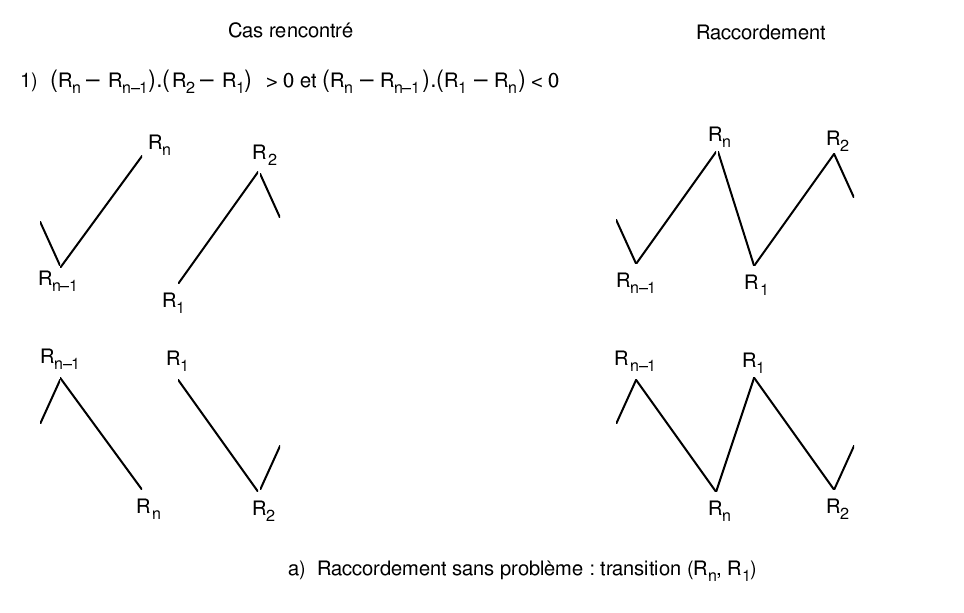
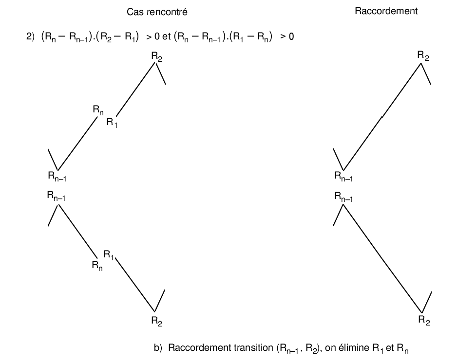
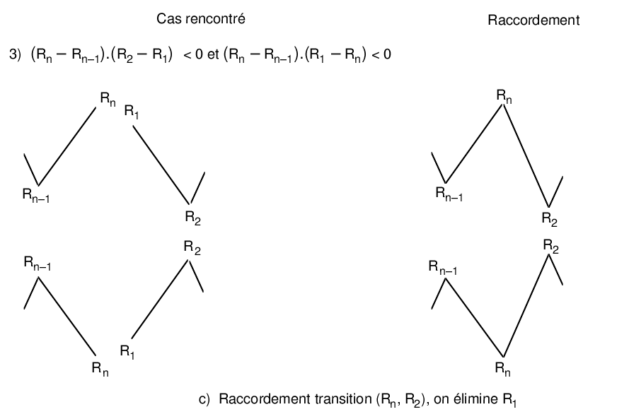
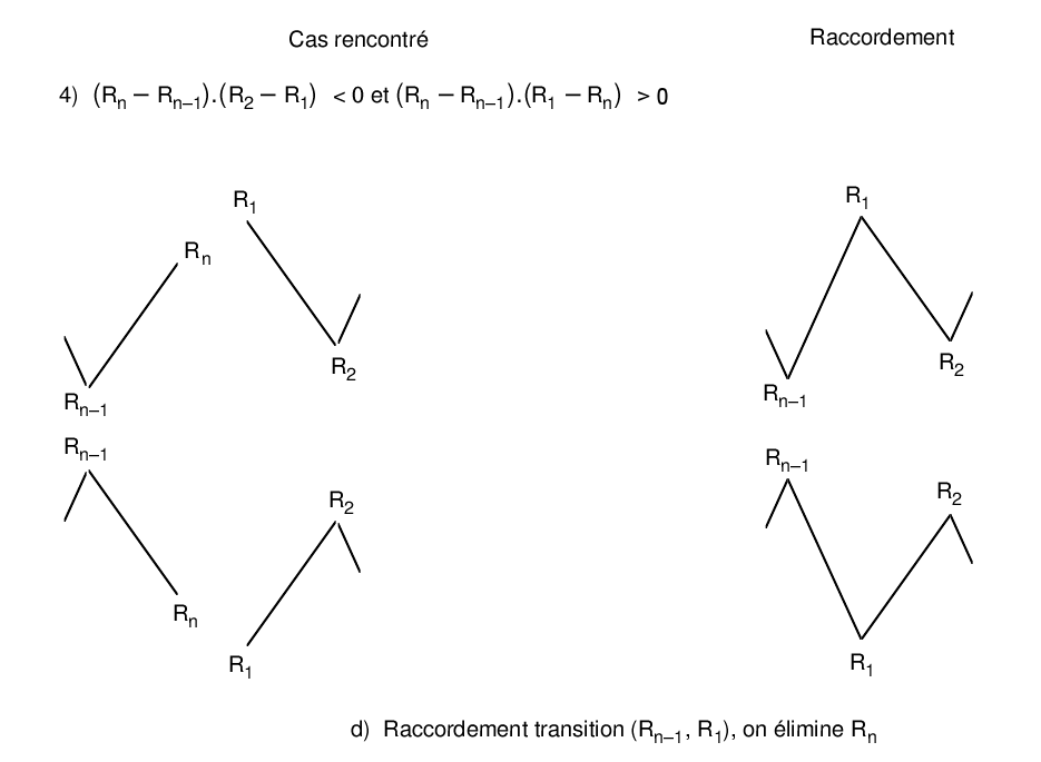
The last point of the residue is followed by the first point of the cycle. As a result, the points considered may no longer appear as extremes. In the event that this happens, they should be eliminated. Eight different cases are encountered. To deal with them explicitly, let’s call \({R}_{1}\) and \({R}_{2}\) the first two points of the residue and \({R}_{n-1}\) and \({R}_{n}\) its last two points.
Notes:
Recommendation AFNOR A 03-406 also refers to a possible pre-processing of the signal, which would consist of signal filtering (suppression of interference) and a quantification of the loading history.
Signal filtering is possible at the user’s request (see [§2.1]). Extraction of peaks).
Quantifying the signal can be useful for the rapid exploitation of fatigue analysis results. In practice, signal quantization consists in dividing the maximum extent of the signal into classes of intervals of constant width called steps, and reducing to a value representative of a given class (its average value in general) all the values located in this class. As for this possibility of pre-processing the signal, it is not available in Code_Aster.
In the special case where the load history is constant (for example, average load applied), Code_Aster will count the entire load history as a zero amplitude cycle.
In order to illustrate the method and to specify the points that would remain unclear, we consider the following loading story (which for example is considered to be of the constraint type):
Point number |
1 |
2 |
3 |
3 |
3 |
3 |
4 |
4 |
5 |
6 |
9 |
10 |
11 |
12 |
13 |
13 |
13 |
13 |
13 |
13 |
14 |
15 |
Instant |
||||||||||||||||||||||
Loading |
—10. |
—70. |
—50. |
—30. |

The method of RAINFLOW therefore leads, in this example, (see [§Annexe1], for details of the steps of the algorithm) to the determination of 7 elementary cycles defined by the maximum value and the minimum value of the load, for each cycle.
Cycle 1: |
VALMAX = 20. |
|
Cycle 2: |
VALMAX = 25. |
|
Cycle 3: |
VALMAX = 30. |
|
Cycle 4: |
VALMAX = 40. |
|
Cycle 5: |
VALMAX = 50. |
|
Cycle 6: |
VALMAX = 60. |
|
Cycle 7: |
VALMAX = 80. |
|
Notes:
The damage calculation does not take into account the order in which the elementary loading cycles appear, it is inconsequential to rearrange the loading history.
For Taheri methods, the order of application of the elementary loading cycles is taken into account, so it is necessary to be very careful when using such a method of counting cycles. It is advisable, for the calculation of damage by Taheri methods, to use the so-called « natural » counting method [§2.2.3].
2.2.2. Method RCC_M#
This method consists in forming the elementary stress cycles starting with those that cause the greatest variations.
Thus, for a loading story comprising \(N\) points, \(N/2\) elementary cycles are determined if \(N\) is even and \(N/2+1\) if \(N\) is odd.
The algorithm is divided into two steps. The first step is to order the loading history from the smallest to the largest value of the stress, or deformation.
For its part, the second step consists in forming the elementary cycles with the greatest variation in the value of the stress, or of the deformation.
On the rearranged \(\text{ch}(t)\) loading story, the elementary cycles are defined by:
\(\{\begin{array}{ccc}\text{VALMAX}={\text{ch}}_{N+1-i}& & \text{pour}i=\mathrm{1,}\text{}N/2\\ \text{VALMIN}\text{}=\text{}{\text{ch}}_{i}& & \end{array}\)
If \(N\) is odd we determine an additional cycle defined by:
\(\{\begin{array}{ccc}\text{VALMAX}={\text{ch}}_{N/2+1}& & \text{si}{\text{ch}}_{N/2+1}>{\text{ch}}_{m}\\ \text{VALMIN}=–{\text{ch}}_{N/2+1}+2\ast {\text{ch}}_{m}& & \end{array}\)
and
\(\{\begin{array}{ccc}\text{VALMAX}={\text{ch}}_{N/2+1}& & \text{sinon}\\ \text{VALMIN}=–{\text{ch}}_{N/2+1}+2\ast {\text{ch}}_{m}& & \end{array}\)
where \({\text{ch}}_{m}=\) mean stress or mean load deformation = \(\frac{1}{N}\sum _{1}^{N}{\text{ch}}_{i}\).
To illustrate method RCC_M let’s consider the same example as that used for method RAINFLOW (whose loading was considered to be of the constraint type).
Point number |
1 |
2 |
3 |
3 |
3 |
3 |
4 |
4 |
5 |
6 |
9 |
10 |
11 |
12 |
13 |
13 |
13 |
13 |
13 |
13 |
14 |
15 |
Instant |
||||||||||||||||||||||
Loading |
—10. |
—70. |
—50. |
—30. |

The first step, which consists in ordering the history of the load, from the smallest to the largest value of the load, leads to the following storage:
Point no. |
9 |
11 |
13 |
13 |
13 |
3 |
3 |
1 |
15 |
12 |
14 |
7 |
10 |
2 |
2 |
2 |
6 |
6 |
6 |
4 |
8 |
Loading |
—70. |
—50. |
—30. |
—10. |
Since the loading history consists of 15 points, method RCC_M determines 8 elementary cycles:
Cycle 1: |
VALMAX = 80. |
and |
VALMIN = —70. |
|
Cycle 2: |
VALMAX = 60. |
and |
VALMIN = —50. |
|
Cycle 3: |
VALMAX = 50. |
and |
VALMIN = —30. |
|
Cycle 4: |
VALMAX = 40. |
and |
VALMIN = —10. |
|
Cycle 5: |
VALMAX = 30. |
and |
VALMIN = 0. |
|
Cycle 6: |
VALMAX = 30. |
and |
VALMIN = 0. |
|
Cycle 7: |
VALMAX = 25. |
and |
VALMIN = 20. |
|
Cycle 8: |
VALMAX = 20. |
and |
VALMIN = 6. |
because \(({\sigma }_{m}=\frac{1}{N}\sum _{1}^{N}{\sigma }_{i}=6\text{.})\) |
Note:
This method of counting cycles absolutely does not take into account the order in which the cycles appear, and systematically orders the elementary cycles by decreasing amplitude. This method must be used with vigilance for the calculation of damage by Taheri methods, the particularity of which is to take into account the order in which the loading cycles are applied. For the calculation of damage using Taheri methods, it is strongly recommended to use the so-called « natural » cycle counting method [§2.2.3].
2.2.3. « Natural » method#
This method consists in generating the cycles in the order in which they appeared in the load history.
Thus, for a loading history of \(N+1\) points, we determine \(N/2\) elementary cycles if \(N\) even and \(N/2+1\) elementary cycles if \(N\) odd.
The method consists in relying on three successive points in the loading history.
Note \(X=\mid \text{ch}(i+1)-\text{ch}(i)\mid\) and \(Y=\mid \text{ch}(i+2)-\text{ch}(i+1)\mid\).
If \(X\ge Y\) we consider that we have encountered an elementary cycle that is defined by the two points \((i)\) and \((i+1)\).
The amplitude of the cycle is given by \(\mathrm{\Delta }\text{ch}=\mid \text{ch}(i+1)-\text{ch}(i)\mid\).
If \(X<Y\) we consider that we have encountered an elementary cycle that is defined by the two points \((i+1)\) and \((i+2)\).
The amplitude of the cycle is given by \(\mathrm{\Delta }\text{ch}=\mid \text{ch}(i+2)-\text{ch}(i+1)\mid\).
When the cycle is extracted we remove the two points \((i)\) and \((i+1)\) from the loading history and we continue with the algorithm.
If the number of \((N+1)\) points in the loading history is odd, the algorithm described above makes it possible to process all the points.
If the number of \((N+1)\) points in the loading story is even, the remaining two points need to be addressed.
These two points are considered to form a cycle defined by the two points \(N\) and \((N+1)\). The amplitude of the cycle is given by \(\Delta \text{ch}=\mid \text{ch}(N+1)-\text{ch}(N)\mid\).
To illustrate this method, consider the same example used for methods RAINFLOW and RCC_M.
Point number |
1 |
2 |
3 |
3 |
3 |
3 |
4 |
4 |
5 |
6 |
9 |
10 |
11 |
12 |
13 |
13 |
13 |
13 |
13 |
13 |
14 |
15 |
Instant |
||||||||||||||||||||||
Loading |
—10. |
—70. |
—50. |
—30. |

Since the loading history consists of 15 points, the « natural » method determines 7 elementary cycles:
Cycle 1: |
VALMAX = 40. |
and |
VALMIN = —10. |
|
Cycle 2: |
VALMAX = 60. |
and |
VALMIN = —10. |
|
Cycle 3: |
VALMAX = 50. |
and |
VALMIN = 20. |
|
Cycle 4: |
VALMAX = 80. |
and |
VALMIN = —70. |
|
Cycle 5: |
VALMAX = 30. |
and |
VALMIN = —70. |
|
Cycle 6: |
VALMAX = 30. |
and |
VALMIN = —50. |
|
Cycle 7: |
VALMAX = 25. |
and |
VALMIN = —30. |
Note:
This method is the one that is strongly recommended to be used when calculating damage using Taheri methods.
2.3. Damage calculation: Wöhler method#
The number of cycles at break is determined by interpolation of the Wöhler curve of the material for a given alternating stress level (to each elementary cycle corresponds a stress amplitude level \(\Delta \sigma =\mid {\sigma }_{\text{max}}-{\sigma }_{\text{min}}\mid\) and an alternating stress \({S}_{\text{alt}}=1/2\Delta \sigma\)).
The damage of an elementary cycle is equal to the inverse of the number of cycles at break \(D=1/N\).
In the case of a homogeneous uniaxial test with pure (or symmetric) alternating stress, the number of cycles at break is determined from an endurance diagram, also called Wöhler curve or curve \(S-N\).
In the case of geometric defects or elementary cycles of non-zero mean stress, corrections to the Wöhler curve are necessary before determining the number of cycles at break and therefore the elementary damage.
2.3.1. Endurance diagram#
The endurance diagram, also called Wöhler curve or curve \(S-N\) (stress-number of cycles at break curve), is obtained experimentally by subjecting test specimens to periodic (generally sinusoidal) force cycles of normal amplitude \(\sigma\) and constant frequencies, and by noting the number of cycles \(N\) at the end of which failure occurs.
The Wöhler curve is therefore defined for a given material and takes the form:

where \({S}_{\text{alt}}\) = the alternating stress of the cycle = \(\frac{1}{2}\mid {\mathrm{\sigma }}_{\text{max}}-{\mathrm{\sigma }}_{\text{min}}\mid\)
There are three areas on this curve:
a zone of oligocyclic fatigue, under high stress, where rupture occurs after a very small number of alternations,
a zone of fatigue or limited endurance, where failure is reached after a number of cycles that increases when the stress decreases,
an unlimited endurance zone or safety zone, under low stress, for which failure does not occur before a given number of cycles greater than the expected lifetime for the part.
There are numerous expressions for the endurance diagram:
The oldest is that of Wöhler:
\(\text{ln}(N)=a-{\mathrm{bS}}_{\text{alt}}\) eq 2.3.1-1
where \(N\) is the number of cycles at break,
\({S}_{\text{alt}}\) the alternating stress applied,
\(a\) and \(b\) are two characteristics of the material.
This analytic expression does not take a good account of a horizontal or asymptotic branch of the complete S-N curve, but it gives an often very good representation of the mean part of the curve.
As early as 1910, Basquin proposed the formula:
\(\text{ln}(N)=a-b\text{ln}({S}_{\text{alt}})\) eq 2.3.1-2
to take into account the curvature of the Wöhler curve that connects the descending branch to the horizontal branch.
\(D\) = damage of an elementary cycle = \(1/N=A{S}_{\text{alt}}^{\beta }\) where \(A={e}^{-a}\) and \(\beta =b\).
Another analytic form of the Wöhler curve is proposed in POSTDAM to take into account the curve outside the singular zone:
\({S}_{\text{alt}}=1/2({E}_{C}/E)\Delta \sigma\) eq 2.3.1-3
\(\begin{array}{cc}\mathrm{où}& {E}_{C}=\text{Module d'Young associé à la courbe de fatigue du matériau,}\\ & E=\text{Module d'Young utilisé pour déterminer les contraintes}\text{.}\\ & X={\text{LOG}}_{\text{10}}({S}_{\text{alt}})\\ & N={\text{10}}^{\mathrm{a0}+\mathrm{a1X}+a2{X}^{2}+{\mathrm{a3X}}^{3}}\\ & D=\{\begin{array}{ccc}1/N& \text{si}{S}_{\text{alt}}\ge {S}_{l}& \text{où}{S}_{l}\text{est la limite d'endurance du matériau}\\ 0\text{.}& \text{sinon}& \end{array}\end{array}\)
Note:
If we taken \(\mathrm{a2}=\mathrm{a3}=0\text{et}{E}_{C}/E=1\) we find Basquin’s formula.
The user can enter the Wöhler curve into the DEFI_MATERIAU [U4.43.01] operator in three distinct forms:
a discretized form point by point (keyword WOHLER under the keyword factor FATIGUE in DEFI_MATERIAU).
In this case, the Wöhler curve is a function that gives the number of cycles at break \(N\) as a function of the alternating stress \({S}_{\text{alt}}\) and for which the user chooses the interpolation mode:
“LOG” —-> logarithmic interpolation on the number of cycles at break and on the alternating stress (piecewise Basquin formula),
“LIN” —-> linear interpolation on the number of cycles at break and on the alternating stress (this interpolation is not recommended because the Wöhler curve is absolutely not linear in this coordinate system).
“LIN”, “LOG” logarithmic interpolation on the number of cycles at break and linear interpolation on the alternating stress, which leads to the expression given by Wöhler.
The user must also choose the type of extension of the function to the right and to the left (if it is necessary to interpolate the function at a point not authorized by the definition of the function, the program is stopped by fatal error).
an analytical form of Basquin (keywords A_ BASQUIN and BETA_BASQUIN under the keyword factor FATIGUE in DEFI_MATERIAU)
\(D=A{S}_{\text{alt}}^{\mathrm{\beta }}\) The constants \(A\) and \(\beta\) used in this formula must be entered by the user (in accordance with the code POSTDAM).
an analytical form outside of a singular zone
\(\begin{array}{}{S}_{\text{alt}}=\text{contrainte alternée}=1/2({E}_{C}/E)\mathrm{\Delta \sigma }\\ X={\text{LOG}}_{\text{10}}({S}_{\text{alt}})\\ N={\text{10}}^{\mathrm{a0}+\mathrm{a1}X+\mathrm{a2}{X}^{2}+\mathrm{a3}{X}^{3}}\\ D=\{\begin{array}{ccc}1/N& \text{si}{S}_{\text{alt}}\ge {S}_{l}& \text{où}{S}_{l}\text{est la limite d'endurance du matériau}\\ 0\text{.}& \text{sinon}& \end{array}\end{array}\)
The user must enter:
\({E}_{C}\) = |
Young’s modulus associated with the material fatigue curve (keyword E_ REFEsous the keyword factor FATIGUE in DEFI_MATERIAU) |
\(E\) = |
Young’s modulus used to determine constraints (keyword E under the keyword factor ELAS in DEFI_MATERIAU), |
the constants of the material \(\mathrm{a0},\mathrm{a1},\mathrm{a2}\mathrm{et}\mathrm{a3}\) (keywords A0, A1, A2 and A3 under the keyword factor FATIGUE in DEFI_MATERIAU)
and \({S}_{l}\) the material’s endurance limit (keyword SL under the keyword factor FATIGUE in DEFI_MATERIAU).
Note:
This damage expression is available in the same form in software POSTDAM.
2.3.2. Influence of geometric parameters on endurance#
2.3.2.1. Stress concentration coefficient#
Depending on the geometry of the part, it may be necessary to weight the value of the stress applied by the stress concentration coefficient \({K}_{T}\text{.}\text{}{K}_{T}\). \({K}_{T}\) is a coefficient that is a function of the geometry of the part, the geometry of the defect, and the type of load.
This coefficient is given by the user under the keyword \({K}_{T}\) of the keyword factor COEF_MULT.
It is used to apply a \({K}_{T}\) ratio homothetic to the loading history, which is equivalent to multiplying all values in the loading history by the \({K}_{T}\) coefficient.
(The damage calculation will be based on a loading story \(\mathrm{\sigma }(t)={K}_{T}\times \mathrm{\sigma }(t)\)).
2.3.2.2. Elasto-plastic concentration coefficient#
It may also be necessary to weight the value of the stress applied by the elasto-plastic concentration coefficient \({K}_{e}\).
The elasto-plastic concentration coefficient \({K}_{e}\) (referred to in articles B3234.3 and B3234.5 of RCC_M [bib4]) is defined as being the ratio between the actual deformation amplitude and the fictional deformation amplitude determined by the elastic analysis.
An acceptable value for the \({K}_{e}\) coefficient can be determined by [bib4]:
\(\{\begin{array}{ccccc}{K}_{e}=1& \text{si}& & \mathrm{\Delta \sigma }<& {\mathrm{3S}}_{m}\\ {K}_{e}=1+(1-n)(\mathrm{\Delta \sigma }/{\mathrm{3S}}_{m}-1)/(n(m-1))& \text{si}& {\mathrm{3S}}_{m}& <\mathrm{\Delta \sigma }<& {\mathrm{3mS}}_{m}\\ {K}_{e}=1/n& \text{si}& {\mathrm{3mS}}_{m}& <\mathrm{\Delta \sigma }& \end{array}\)
where \({S}_{m}\) is the maximum allowable stress,
and \(n\) and \(m\) two constants that depend on the material.
The elasto-plastic factor \({K}_{e}\) is a load homothetic ratio. This factor depends on the magnitude of the load. It is applied, cycle by cycle, on the values of the maximum and minimum stress of each cycle.
Data \({S}_{m}\), \(n\), and \(m\) are entered under the keywords SM_KE_RCCM, N_ KE_RCCM, and M_ KE_RCCM under the keyword factor FATIGUE in DEFI_MATERIAU.
The user requests that the elasto-plastic concentration factor be taken into account by indicating CORR_KE: “RCCM” in POST_FATIGUE [U4.83.01].
2.3.3. Influence of mean stress#
If the part is not subjected to pure or symmetric alternating stresses, i.e. if the mean stress of the cycle is not zero, the resistance to dynamic stresses of the material (its endurance limit) decreases.
The Wöhler curve is therefore weighted to calculate the number of effective breaking cycles using various diagrams.
The Haigh diagram makes it possible to determine the evolution of the endurance limit as a function of the mean stress \({\mathrm{\sigma }}_{m}\) and the alternating stress \({S}_{\text{alt}}\).

From a cycle \(({S}_{\text{alt}},{\mathrm{\sigma }}_{m})\) identified in the signal, the value of the corrected alternating stress \({S}_{\text{alt}}^{\text{'}}\) is calculated.
\(\begin{array}{cc}\text{Si l'on utilise la droite de Goodman}& {S}_{\text{alt}}^{\text{'}}=\frac{{S}_{\text{alt}}}{1-\frac{{\mathrm{\sigma }}_{m}}{{S}_{u}}}\\ \text{Si l'on utilise la parabole de Gerber}& \begin{array}{}\\ {S}_{\text{alt}}^{\text{'}}=\frac{{S}_{\text{alt}}}{1-{(\frac{{\mathrm{\sigma }}_{m}}{{S}_{u}})}^{2}}\end{array}\end{array}\)
If we use the Goodman line: \({S}_{\text{alt}}^{\text{'}}=\frac{{S}_{\text{alt}}}{1-\frac{{\sigma }_{m}}{{S}_{u}}}\)
If we use Gerber’s parable: \({S}_{\text{alt}}^{\text{'}}=\frac{{S}_{\text{alt}}}{1-{(\frac{{\sigma }_{m}}{{S}_{u}})}^{2}}\)
Note that the latter does not differentiate between the mean tensile and compressive stress.
where \({S}_{u}\) is the breaking limit of the material.
The influence of the average stress is only taken into account at the user’s request (keyword CORR_HAIG).
Note:
If the Wöhler curve is defined by the analytical form outside the singular zone [éq2.3.1‑3], ranges of stress variation that are below the endurance limit may be greater than this limit. To avoid this, we correct the endurance limit \({S}_{l}\) by taking a corrected endurance limit [bib5]:
\({S}_{l}^{\text{'}}=\frac{{S}_{l}}{1-\frac{{\sigma }_{m}}{{S}_{u}}}\) for Goodman’s right
\({S}_{l}^{\text{'}}=\frac{{S}_{l}}{1-{(\frac{{\sigma }_{m}}{{S}_{u}})}^{2}}\) for the Gerber parable
2.4. Calculation of damage: Manson-Coffin method#
The field of application of the Manson-Coffin method [bib1] is oligocyclic plastic fatigue, which, as its name suggests, has two fundamental characteristics:
it is plastic, that is to say that a significant plastic deformation occurs during each cycle,
it is oligocyclic, that is to say that the materials have a finite endurance to this type of stress.
To describe the behavior of materials under oligocyclic plastic fatigue, alternating imposed deformation tests are used.
In the case of a homogeneous uniaxial test with alternating deformation, the number of cycles at failure is determined from a resistance diagram, which relates the variation in deformation to the number of cycles causing the failure.
In the resistance diagram, total, elastic, and plastic deformations are separated. These diagrams are still known under the name of Coffin-Manson who proposed them in 1950.

The relationships \(\frac{\Delta {\varepsilon }_{e}}{2}-\text{ln}(N)\) and \(\frac{\Delta {\varepsilon }_{p}}{2}-\text{ln}(N)\) are right. For its part, the \(\frac{\Delta {\varepsilon }_{t}}{2}-\text{ln}(N)\) relationship has a curvature towards positive deformations.
It has been shown that a power relationship relates plastic deformation \(({\mathrm{\Delta \varepsilon }}_{p})\) and elastic deformation \(({\mathrm{\Delta \varepsilon }}_{e})\) to the number of cycles at break, which leads to the following relationships:
\(\begin{array}{}\Delta {\varepsilon }_{p}=A{N}^{-a}\\ \Delta {\varepsilon }_{e}=B{N}^{-b}\\ \Delta {\varepsilon }_{t}=A{N}^{-a}+B{N}^{-b}\end{array}\)
where \(a\) and \(b\) are two characteristics of the material (in general \(a\) is close to \(\mathrm{0,5}\) and \(b\) is close to \(\mathrm{0,12}\)); \(A\) and \(B\), two constants of the material.
The user can introduce the Manson-Coffin curve in a unique mathematical form: discretized form point by point. It is a function that gives the number of cycles at break \(N\) as a function of the deformation amplitude \((\Delta {\varepsilon }_{})\).
As for the Wöhler curve, the user can choose the interpolation mode based on the number of cycles at break and on the amplitude of deformation.
The type of extension of the function to the right and to the left is also up to the user.
The damage of an elementary cycle is equal to the inverse of the number of cycles at break \(D=1/N\).
2.5. Damage calculation: Taheri method#
The damage calculation methods proposed by Taheri [bib12] are two in number: they will be called Taheri-Manson and Taheri-Mixte respectively. These methods apply to loads characterized by a scalar component such as deformation.
The particularity of these methods is that they take into account the order in which the elementary loading cycles are applied to the structure. For this reason, care should be taken when choosing the method for counting cycles. It is strongly recommended to use the counting method known as the « natural » method [§2.2.3].
2.5.1. Taheri-Manson method#
Let n elementary cycles of half-amplitude \(\frac{{\mathrm{\Delta \varepsilon }}_{1}}{2},\cdots \frac{{\mathrm{\Delta \varepsilon }}_{n}}{2}\) be.
The value of the elementary damage of the first cycle is determined by interpolation on the Manson-Coffin curve of the material.
The calculation of the elementary damage of the following cycles is carried out by the algorithm:
if \(\frac{{\mathrm{\Delta \varepsilon }}_{i+1}}{2}\ge \frac{{\mathrm{\Delta \varepsilon }}_{i}}{2}\)
the value of the elementary damage of cycle \((i+1)\) is determined by interpolation on the Manson-Coffin curve of the material.
if \(\frac{{\mathrm{\Delta \varepsilon }}_{i+1}}{2}<\frac{{\mathrm{\Delta \varepsilon }}_{i}}{2}\)
we determine:
\(\frac{{\mathrm{\Delta \sigma }}_{i+1}}{2}={F}_{\text{NAPPE}}(\frac{{\mathrm{\Delta \varepsilon }}_{i+1}}{2},\underset{j<i}{\text{Max}}(\frac{{\mathrm{\Delta \varepsilon }}_{j}}{2}))\)
then
\(\frac{\Delta {\varepsilon }_{i+1}^{\ast }}{2}={F}_{\text{FONC}}(\frac{\Delta {\sigma }_{i+1}}{2})\).
\({F}_{\text{NAPPE}}\) is the cyclic work hardening curve with cyclic pre-working of the material.
\({F}_{\text{FONC}}\) is the cyclic work hardening curve of the material.
The damage value of cycle \((i+1)\) is determined by interpolation of \(\frac{{\mathrm{\Delta \varepsilon }}_{i+1}^{\ast }}{2}\) on the Manson-Coffin curve of the material.
Note:
If all the cycles applied are arranged by increasing value of the deformation amplitude, this method is identical to the Manson-Coffin method.
2.5.2. Taheri-Mixte method#
Let n elementary cycles, of half-amplitude \(\frac{{\mathrm{\Delta \varepsilon }}_{1}}{2},\cdots \frac{{\mathrm{\Delta \varepsilon }}_{n}}{2}\).
The value of the elementary damage of the first cycle is determined by interpolation on the Manson-Coffin curve of the material.
The calculation of the elementary damage of the following cycles is carried out by the algorithm:
if \(\frac{{\mathrm{\Delta \varepsilon }}_{i+1}}{2}\ge \frac{{\mathrm{\Delta \varepsilon }}_{i}}{2}\)
the value of the elementary damage of cycle \((i+1)\) is determined by interpolation on the Manson-Coffin curve of the material.
if \(\frac{{\mathrm{\Delta \varepsilon }}_{i+1}}{2}<\frac{{\mathrm{\Delta \varepsilon }}_{i}}{2}\)
we determine:
\(\frac{{\mathrm{\Delta \sigma }}_{i+1}}{2}={F}_{\text{NAPPE}}(\frac{{\mathrm{\Delta \varepsilon }}_{i+1}}{2},\underset{j<i}{\text{Max}}(\frac{{\mathrm{\Delta \varepsilon }}_{j}}{2}))\)
where \({F}_{\text{NAPPE}}\) is the cyclic work hardening curve with cyclic pre-work hardening of the material.
The damage value for cycle \((i+1)\) is obtained by interpolating \(\frac{{\mathrm{\Delta \sigma }}_{i+1}}{2}\) onto the material’s Wöhler curve.
Note:
If all the cycles applied to the structure are arranged by increasing value of the deformation amplitude, this method is identical to the Manson-Coffin method.
The damage of an elementary cycle is equal to the inverse of the number of cycles at break \(D=1/N\).
2.6. Calculation of total damage#
The simplest and best known approach for determining the total damage of a part subjected to \({n}_{i}\) cycles of alternating stress \({S}_{\text{alt}}\) or alternating deformation \({E}_{\text{alt}}\) is the linear damage rule proposed by Miner:
\(\text{Di}=\frac{{n}_{i}}{{N}_{i}}\)
During operation, the structures are subjected to various loads of different amplitudes. The fatigue suffered is due to the accumulation of elementary damage and the total damage is calculated using Miner’s accumulation rule [bib6]:
\({D}_{\text{total}=}\sum _{i}^{}\frac{{n}_{i}}{{N}_{i}}\)
In the case of Wöhler and Manson-Coffin, this law assumes that the damage increases linearly with the number of cycles imposed and that it is independent of the loading level and the order in which the loading levels are applied (whereas experimentally, it is shown that the order of application of the load is an important factor for the life of the material).
The calculation of the total damage is requested by the user with the keyword CUMUL.
The methods proposed by Taheri take into account the order in which the load is applied, in calculating the elementary damages associated with each cycle.
2.7. Conclusion#
For methods based on uniaxial tests, the calculation of the total damage suffered by a part subjected to a loading history is divided into several steps:
extraction of the peaks of the loading history, to arrive at a simpler story,
extraction of elementary cycles from the loading history by a cycle counting method,
calculation of the elementary damage associated with each elementary cycle based on the real history of the load,
possibly (and for the Wöhler method), correction of the loading by a stress concentration coefficient \({K}_{T}\),
possibly (and for the Wöhler method), correction of the loading by an elasto-plastic concentration coefficient \({K}_{e}\),
possibly (and for the Wöhler method), Haigh correction to take into account the non-zero value of the mean stress,
calculation of total damage, using a linear accumulation rule.