2. Definition of law CZM_TURON#

2.1. Definitions#

Let’s start by introducing the model parameters. We have:

the critical surface energy densities in pure normal mode and in pure tangential mode, noted \({G}_{c,N}\) (keyword GC_N) and \({G}_{c,T}\) (keyword GC_T) which reflect the energy cost of cracking in each of the two modes;
the critical stress at failure noted \({\mathrm{\sigma }}_{N}^{c}\) (keyword SIGM_C_N) and \({\mathrm{\sigma }}_{T}^{c}\) (keyword SIGM_C_T);
the initial stiffness of the interface \(K\) (keyword K);
the parameter

the Benzeggagh-Kenane criterion (keyword ETA_BK);

the dimensionless parameter C_ RUPT which makes it possible to define a « post-break » residual stiffness (when the element is completely damaged and the cohesive stress is zero), as a fraction of the initial stiffness. It is set to 0.001 by default and cannot exceed 0.1;
the parameter CRIT_INIT which allows you to choose the type of damage initiation criterion, among “YE” (elliptical criterion) or “TURON” (Benzeggagh-Kenane type criterion).

The material parameters themselves, namely GC_N, GC_T,,,, SIGM_C_N,,, SIGM_C_T, K and ETA_BK, are to be identified on the basis of standard quasistatic tests. For example, as part of the simulation of a glued joint, the adhesive being modeled with the cohesive zone model, the parameters will be identified by carrying out the following tests on « sandwich » specimens:

test DCB (« Double Cantilever Beam ») which stresses the joint in pure normal mode makes it possible to identify the parameters GC_Net SIGM_C_N;
test ENF (« End-notched flexure »), corresponding to 3-point flexure, stresses the joint in pure tangent mode and makes it possible to identify the parameters GC_Tet SIGM_C_T;
test MMB (« Mixed-mode bending ») is a combination of the two previous tests and makes it possible to subject the joint to a mixed loading, the mixing rate being in the hands of the experimenter who can adjust the device. In addition to the previous tests, it is used to set the parameter ETA_BK.

With regard to the parameter \(K\), it is generally observed that it has little influence on the simulated global response and that it is therefore difficult to identify it by adjusting the numerical and experimental curves. In practice, it is often assumed ad hoc.

Note:

We adopt the following notations: for any vector \(x\) we note:

\(x={x}_{N}N+{x}_{{T}_{1}}{T}_{1}+{x}_{{T}_{2}}{T}_{2}\)

\({x}_{T}={x}_{{T}_{1}}{T}_{1}+{x}_{{T}_{2}}{T}_{2}\)

\(⟨x⟩=⟨{x}_{N}⟩N+{x}_{{T}_{1}}{T}_{1}+{x}_{{T}_{2}}{T}_{2}\) with \(⟨{x}_{i}⟩=\mathit{max}({x}_{i},0)\)

\(\Vert x\Vert =\sqrt{x\mathrm{.}x}\) and \({\Vert x\Vert }_{+}=\sqrt{⟨x⟩\mathrm{.}⟨x⟩}\)

In particular, we note \(\mathrm{\lambda }={\Vert \mathrm{\Delta }\Vert }_{+}\) the equivalent displacement of the cohesive element and \({\mathrm{\lambda }}_{T}=\Vert {\mathrm{\Delta }}_{T}\Vert\) the norm of the tangential jump.

Finally, we call:

\({\mathrm{\Delta }}^{0}\) the value that the equivalent jump must wait for the damage to occur. It is therefore called damage initiation jump;
\({\mathrm{\Delta }}^{f}\) the value that the equivalent jump must reach for the element to break. It is therefore called crack propagation jump (but this name should not mislead the reader: models with law CZM do not present cracks per se, for example, directly meshed or well defined by level sets).

The initial stiffness \(K\) makes it possible to regulate the free energy in 0. This law is therefore a regularized model law. Note that in the case where the interface is supposed to be infinitely rigid, for example when the interface models a crack path in a fragile material, then the initial stiffness must be small enough for the energy to be well regulated, but this can in turn lead to an overall relaxation of the structure that is not physical.

In the context of the modeling of an interface with a certain « flexibility » which is physical (for example a layer of glue between two adherents that will deform elastically before starting to be damaged), this problem does not arise.

It should be remembered that there should not be too great a difference in stiffness between cohesive elements of type JOINTet and directly neighboring elements (generally volume), at the risk of encountering problems in conditioning the system’s stiffness matrix, specific to this type of element [5]. In practice, it can be verified that the parameter \(K\) and the quantity \(\frac{E}{{h}_{\mathit{elem}}}\) are of the same order of magnitude, \(E\) being the Young’s modulus of the adherent and \({h}_{\mathit{elem}}\) being the size of the cells adjacent to the joined elements. To a certain extent, it is possible to adapt the size of the adjacent cells. But if the packaging problems cannot be solved given too much difference between the material properties of the cohesive interface and the adherent, we will rather turn to elements of the INTERFACE [5, 6] type, on which certain laws CZM [7] are available, on which certain laws [] are available.

2.2. Behavioral equations#

In this part we present the surface energy \(\mathrm{\Psi }\) as well as the stress vector that

drifting out. The proposed formulation ensures the irreversibility of the damage.

2.2.1. Surface free energy#

The free energy per unit area \(\Psi\), defined on a discontinuity \(\mathrm{\Gamma }\), depends on the jump displacement vector between the lips of the crack \(\mathrm{\Delta }\) (noted \(\mathrm{\Delta }\) to simplify the writing) and on an internal variable that manages the irreversibility of the crack.

First of all, we define the variable \(v\) which memorizes the largest jump norm (equivalent displacement) reached during the opening. Its law of evolution between two successive loading increments - and + is written as:

\({v}^{+}=\mathit{max}({\mathrm{\lambda }}_{+},{v}^{-})\)

We also define the threshold variable noted \(r\) which gives the minimum jump to be reached in order to (re) start damaging:

\({r}^{+}=\mathit{max}({\mathrm{\Delta }}^{\mathrm{0,}}{v}^{-})\)

Finally, let’s define the damage variable \(d\), whose law of evolution will be given below. The item is healthy when \(d=0\) is completely damaged, broken, when \(d=1\).

It should be noted that from the thermodynamic point of view, the variable \(d\) is used here, which is the internal variable of the behavior. On the other hand, from the point of view of the numerical implementation, the variable \(v\) will be used as an internal variable, the other variables \(r\) and \(d\) being calculated from \(v\).

We give ourselves the following free energy per unit area:

(2.1)#\[ \ mathrm {\ Psi} (\ mathrm {\ Delta}, d) = (1-d) {\ mathrm {\ Psi}} ^ {0} (\ mathrm {\ Delta})\]

with \({\mathrm{\Psi }}^{0}(\mathrm{\Delta })=\frac{1}{2}{\mathrm{\Delta }}_{i}{D}_{\mathit{ij}}^{0}{\mathrm{\Delta }}_{j}\) for \(i,j=\mathrm{1,}3\)

\({\mathrm{\Psi }}^{0}\) being a convex function in the space of movement jumps.

The negative values of \({\mathrm{\Delta }}_{N}\) do not make sense because the interpenetration of the lips is made impossible by contact. To prevent interpenetration after complete de-cohesion, it is proposed to modify the equation according to the following form:

\(\mathrm{\Psi }(\mathrm{\Delta },d)=(1-d){\mathrm{\Psi }}^{0}(\mathrm{\Delta })-d{\mathrm{\Psi }}^{0}({\mathrm{\delta }}_{Ni}⟨-{\mathrm{\Delta }}_{N}⟩)\)

where \({\mathrm{\delta }}_{\mathit{ij}}\) is the Kronecker symbol.

2.2.2. Expression of constraint#

The behavioral equations are obtained by differentiating free energy with respect to jumps in movement:

(2.2)#\[ {\ mathrm {\ tau}} _ {i} =\ frac {\ partial\ mathrm {\ Psi}} {\ partial {\ mathrm {\ Delta}} _ {i}} = (1-d) {D}} = (1-d) {D}} _ {D} _ {D} _ {D} _ {\ mathit {ij}} _ {\ mathit {ij}}} ^ {0}} {\ mathrm {\ Delta}}} _ {j} -d {D}} = (1-d) {D} {D}} _ {D} _ {D} _ {D} _ {D} _ {\ mathit {ij}} _ {\ mathit {ij}}}} ^ {0} {\ mathrm {\ delta}}} _ {\ mathit {Nj}} ⟶- {\ mathrm {\ Delta}}} _ {N}\]

where \({D}_{\mathit{ij}}^{0}={\mathrm{\delta }}_{\mathit{ij}}K\) is the initial stiffness tensor, with \(K\) the penalization stiffness.

Assuming \(N\equiv 1\) and \(({T}_{\mathrm{1,}}{T}_{2})\equiv (\mathrm{2,}3)\), the equation can be written in a vector way:

\(\mathrm{\tau }=\left\{\begin{array}{c}{\mathrm{\tau }}_{1}\\ {\mathrm{\tau }}_{2}\\ {\mathrm{\tau }}_{3}\end{array}\right\}=(1-d)K\left\{\begin{array}{c}{\mathrm{\Delta }}_{1}\\ {\mathrm{\Delta }}_{2}\\ {\mathrm{\Delta }}_{3}\end{array}\right\}-dK\left\{\begin{array}{c}⟨-{\mathrm{\Delta }}_{1}⟩\\ 0\\ 0\end{array}\right\}\)

The energy dissipated during the evolution of the damage is noted \(\mathrm{\Xi }\) and is obtained by differentiating the free energy by the internal damage variable:

\(\mathrm{\Xi }=-\frac{\partial \mathrm{\Psi }}{\partial d}\dot{d}\)

The behavior model given in the equation is well evaluated if the damage variable \(d\) can be calculated at each moment of the deformation process, which is possible by giving yourself an initiation criterion and a law of evolution for the damage.

2.2.3. Evolution of damage#

The evolution of the damage is formulated in the form of a threshold function in the space of movement jumps. It is written, in every moment \(t\):

\(F({\mathrm{\lambda }}^{t},{r}^{t})\mathrm{:}={\mathrm{\lambda }}^{t}-{r}^{t}\le 0\) \(\forall t\ge 0\)

where \({r}^{t}\) is the damage threshold at the current point in time.

If we note \({r}^{0}\) is the initial damage threshold then we must have \({r}^{t}\ge {r}^{0}\) at all times. The damage threshold can only increase. The damage is initiated when the displacement jump norm \(\mathrm{\lambda }\) exceeds the initial threshold \({r}^{0}\), which is calculated in particular on the basis of material characteristics.

In the present formulation, an equivalent expression that is easier to process algorithmically will be used:

\(\overline{F}({\mathrm{\lambda }}^{t},{r}^{t})\mathrm{:}=G({\mathrm{\lambda }}^{t})-G({r}^{t})\le 0\) \(\forall t\ge 0\)

where \(G\) is a monotonic scalar function ranging from 0 to 1. The evolution of the threshold and the damage are given by their increases:

\(\dot{r}=\dot{\mathrm{\mu }}\)

\(\dot{d}=\dot{\mathrm{\mu }}\frac{\partial \overline{F}(\mathrm{\lambda },r)}{\partial \mathrm{\lambda }}=\dot{\mathrm{\mu }}\frac{\partial G(\mathrm{\lambda })}{\partial \mathrm{\lambda }}\)

the variable \(\mathrm{\mu }\) being the Lagrange multiplier which makes it possible to define the charge-discharge conditions according to the Kuhn and Tucker relationships:

\(\dot{\mathrm{\mu }}\ge 0\) (a); \(\overline{F}({\mathrm{\lambda }}^{t},{r}^{t})\le 0\) (b); \(\dot{\mathrm{\mu }}\overline{F}({\mathrm{\lambda }}^{t},{r}^{t})=0\) (c)

For educational reasons, we will explicitly integrate Kuhn’s and Tucker’s relationships — a very classical one. To do this, we separate the two « phases »:

Phase A (non-damaging) :

As long as \({\mathrm{\lambda }}^{t}<{r}^{t}\), we have \(G({\mathrm{\lambda }}^{t})<G({r}^{t})\) per growth of the function \(G\), and therefore \(\overline{F}({\mathrm{\lambda }}^{t},{r}^{t})<0\) (consistent with (b)).

By (c), we necessarily have only \(\dot{\mathrm{\mu }}=\dot{r}=0\). So \(r\) remains constant, equal to its value at the beginning of the phase, especially to \({r}^{0}\) if it is the initial moment.

Phase B (damaging) :

If we look at the other expression for (b), where \(\overline{F}({\mathrm{\lambda }}^{t},{r}^{t})=0\), then \({\mathrm{\lambda }}^{t}={r}^{t}\) (we can’t have \({\mathrm{\lambda }}^{t}>{r}^{t}\) otherwise (b) is no longer satisfied). Let’s avoid the case where \(\dot{\mathrm{\mu }}=0\) corresponds to the case where \(\mathrm{\lambda }\) does not evolve. So \(\dot{\mathrm{\mu }}>0\) according to (a) and therefore \(r\) is growing, at the same time as \(\mathrm{\lambda }\). In addition, we can write that \(\dot{d}=\dot{r}\frac{\partial G(r)}{\partial r}\), hence the direct integration of \(d\).

The two phases can alternate according to the loading path, and it is therefore possible to integrate the threshold variable \(r\) and the damage variable \(d\) in the following way:

\({r}^{t}=\mathit{max}({r}^{0},{\mathit{max}}_{s}\mathrm{\lambda })\) \(0\le s\le t\)

\({d}^{t}=G({r}^{t})\)

The damage threshold will be noted in suite \({r}^{0}={\mathrm{\Delta }}^{0}\).

The scalar function \(G\) defines the evolution of the damage variable. For a given mix rate, a function of the following form is proposed:

\(G(\mathrm{\lambda })=\frac{{\mathrm{\Delta }}^{f}(\mathrm{\lambda }-{\mathrm{\Delta }}^{0})}{\mathrm{\lambda }({\mathrm{\Delta }}^{f}-{\mathrm{\Delta }}^{0})}\)

which corresponds to a behavior equation between the stress and the equivalent jump in bilinear form, with \({\mathrm{\Delta }}^{0}\) is the displacement jump at the initiation of the damage, so \({\mathrm{\Delta }}^{0}={r}^{0}\), and \({\mathrm{\Delta }}^{f}\) is the final displacement jump when the damage reaches its maximum value of 1.

We can easily write the equation of the lines in both regimes starting from the equation written with the constraint and the equivalent jump \(\mathrm{\tau }=K(1-d)\mathrm{\lambda }=K(1-G(r))\mathrm{\lambda }\):

in elastic regime (non-damaging phase), with \(\mathrm{\lambda }<r\), we have \(\mathrm{\tau }=K\frac{{\mathrm{\Delta }}^{0}({\mathrm{\Delta }}^{f}-r)}{r({\mathrm{\Delta }}^{f}-{\mathrm{\Delta }}^{0})}\cdot \mathrm{\lambda }\), which corresponds well to the equation of a line since \(r\) does not evolve. In particular, \(\mathrm{\tau }=K\cdot \mathrm{\lambda }\) when \(r={\mathrm{\Delta }}^{0}\);
in a dissipative regime (damaging phase), with \(r=\mathrm{\lambda }\), we have \(\mathrm{\tau }=K\frac{{\mathrm{\Delta }}^{0}{\mathrm{\Delta }}^{f}}{{\mathrm{\Delta }}^{f}-{\mathrm{\Delta }}^{0}}-K\frac{{\mathrm{\Delta }}^{0}}{{\mathrm{\Delta }}^{f}-{\mathrm{\Delta }}^{0}}\cdot \mathrm{\lambda }\), which is indeed the equation of a decreasing affine line.

The bilinear law of this type can be visualized in Figure.

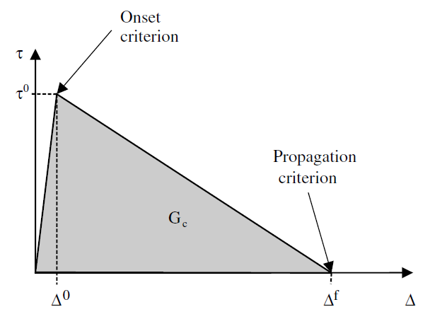
Figure 2.2.1: Bi-linear relationship between stress and equivalent displacement jumps [1]

The jumps in movement at initiation and at propagation are obtained from the corresponding threshold surfaces, which therefore remain to be defined in order to complete the formulation of the behavioral equations.

In this model, these criteria take into account the interaction between normal and tangential loading modes. They therefore depend on the load mix rate defined as follows:

\(\mathrm{\beta }=\frac{{\mathrm{\Delta }}_{T}}{⟨{\mathrm{\Delta }}_{N}⟩+{\mathrm{\Delta }}_{T}}\)

2.2.4. Crack propagation criterion (threshold surface for \(d=1\))#

The proposed mixed mode « crack » propagation criterion is established on the basis of the critical energy restoration rate. For composite joint systems, a common criterion is that of Benzeggagh-Kenane, from the field of fracture mechanics:

\({G}_{c}={G}_{\mathit{Nc}}+({G}_{T,c}-{G}_{N,c}){\left(\frac{{G}_{T}}{{G}_{\mathit{tot}}}\right)}^{\mathrm{\eta }}\)

where \({G}_{\mathit{tot}}={G}_{N}+{G}_{T}\).

It is specified that the criterion, written in the context of fracture mechanics, involves the quantities \({G}_{I,c}\), \({G}_{\mathit{II},c}\) and \({G}_{\mathit{III},c}\), which are the critical energies according to the three classical modes of stress on a crack. But in the context of an interface modelled by an interface law CZM, we can only describe

\({G}_{\mathit{II},c}={G}_{\mathit{III},c}={G}_{T,c}\)

since the definition of what are commonly called modes II and III is based on the crack front. However, here, we are not modeling a crack but a damaging interface, for which we can best define a normal direction and a tangential direction.

We can rewrite this criterion from the jumps in displacement by noting that the critical energy, corresponding to the area under the bilinear curve in Figure, is written as:

\({G}_{c}=\frac{1}{2}K{\mathrm{\Delta }}^{0}{\mathrm{\Delta }}^{f}\)

What gives

\({\mathrm{\Delta }}^{f}=\frac{{\mathrm{\Delta }}_{N}^{0}{\mathrm{\Delta }}_{N}^{f}+({\mathrm{\Delta }}_{T}^{0}{\mathrm{\Delta }}_{T}^{f}-{\mathrm{\Delta }}_{N}^{0}{\mathrm{\Delta }}_{N}^{f}){\left(\frac{{G}_{T}}{{G}_{\mathit{tot}}}\right)}^{\mathrm{\eta }}}{{\mathrm{\Delta }}^{0}}\)

with \({\mathrm{\Delta }}_{N}^{0}\) and \({\mathrm{\Delta }}_{T}^{0}\) the criteria for initiating damage, and \({\mathrm{\Delta }}_{N}^{f}\) and \({\mathrm{\Delta }}_{T}^{f}\) the criteria for propagation in pure modes, calculated from the material data for each mode taking into account the bilinear form of the law (see figure):

\({\mathrm{\Delta }}_{N/T}^{0}=\frac{{\mathrm{\sigma }}_{c,N/T}}{K}\) and \({\mathrm{\Delta }}_{N/T}^{f}=\frac{2{G}_{c,N/T}}{{\mathrm{\sigma }}_{c,N/T}}\)

It should be noted that the mixing rate can be measured by another quantity \(B\) from the energy return rates:

\(B=\frac{{G}_{T}}{{G}_{\mathit{tot}}}\)

The two definitions are linked by the following formula as shown in [1]:

\(B=\frac{{\mathrm{\beta }}^{2}}{1+2{\mathrm{\beta }}^{2}-2\mathrm{\beta }}\)

2.2.5. Criteria for initiating damage (threshold surface for \(d=0\))#

When loading is in pure N or T mode, damage is initiated when the cohesive forces reach their respective critical value \({\mathrm{\sigma }}_{c,N/T}\) (critical stresses). Under mixed loading, it is necessary to take into account an interaction between the modes. There are various models defining the initiation criterion according to the mixing rate. The present law of behavior proposes the Benzeggagh—Kenane model (which is therefore used for both the initiation and propagation criteria — and this with the same power \(\mathrm{\eta }\)). This criterion is referred to as the « Turon criterion », the fact of adopting the same mode coupling equation for initiation and propagation being a choice made by the authors of [1]. Another purely elliptical criterion, designated by the « Ye criterion », is also proposed.

The elliptical criterion of Ye

This is a simple and fairly common criterion. It is based on a quadratic interaction of critical constraints:

\({\left(\frac{⟨{\mathrm{\sigma }}_{N}⟩}{{\mathrm{\sigma }}_{c,N}}\right)}^{2}+{\left(\frac{{\mathrm{\sigma }}_{{T}_{1}}}{{\mathrm{\sigma }}_{c,T}}\right)}^{2}+{\left(\frac{{\mathrm{\sigma }}_{{T}_{2}}}{{\mathrm{\sigma }}_{c,T}}\right)}^{2}=1\)

which is written equivalently in terms of a jump in movement:

\({\left(\frac{⟨{\mathrm{\Delta }}_{N}⟩}{{\mathrm{\Delta }}_{N}^{0}}\right)}^{2}+{\left(\frac{{\mathrm{\Delta }}_{{T}_{1}}}{{\mathrm{\Delta }}_{T}^{0}}\right)}^{2}+{\left(\frac{{\mathrm{\Delta }}_{{T}_{2}}}{{\mathrm{\Delta }}_{T}^{0}}\right)}^{2}=1\)

We therefore have an elliptical criterion in the general anisotropic case where the critical stresses and the associated jumps in displacement are different for the normal and tangent modes.

This criterion is accessible via the value of the keyword CRIT_INIT = “YE” in DEFI_MATERIAU/RUPT_TURON.

The criterion proposed in law CZM_LIN_REGest a particular case of this criterion, and corresponds to the case where the joint is isotropic, that is to say when the normal and tangent properties are equal.

The Turon criterion

It is a Benzeggagh — Kenane criterion for initiation. Although it is difficult to have experimental data validating the choice of one or other of the two criteria mentioned, the idea here is to formulate the initiation and propagation threshold surfaces in a dependent manner. It is written:

\({\mathrm{\sigma }}_{c}^{2}={\mathrm{\sigma }}_{c,N}^{2}+\left({\mathrm{\sigma }}_{c,T}^{2}-{\mathrm{\sigma }}_{c,N}^{2}\right){B}^{\mathrm{\eta }}\)

and, equivalently:

\({({\mathrm{\Delta }}^{0})}^{2}={({\mathrm{\Delta }}_{N}^{0})}^{2}+\left({({\mathrm{\Delta }}_{T}^{0})}^{2}-{({\mathrm{\Delta }}_{N}^{0})}^{2}\right){B}^{\mathrm{\eta }}\)

This criterion is accessible via the keyword value CRIT_INIT = “TURON” in DEFI_MATERIAU.

2.2.6. Criteria visualizations#

To visualize the coupling of the modes by the Ye or Turon criteria, we can look at the threshold surfaces in the travel space, and in particular see the influence of the parameter \(\mathrm{\eta }\) on the threshold.

We recall the normal and tangent properties from the reference [1], characterizing the intralaminar damage of a composite material (i.e. at one of the interfaces between the various « folds » that constitute the composite: it is therefore a damage internal to the composite): it is therefore a damage internal to the composite):

\(K=1.0\times {10}^{15}N/{m}^{3}\)

\({\mathrm{\sigma }}_{c,N}=80\times {10}^{6}\mathit{Pa}\)

\({G}_{c,N}=969N/m\)

\({\mathrm{\sigma }}_{c,T}=100\times {10}^{6}\mathit{Pa}\)

\({G}_{c,T}=1719N/m\)

This gives the following jump in movements at the start of the damage:

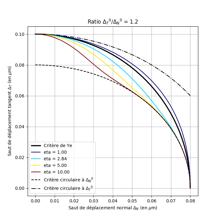
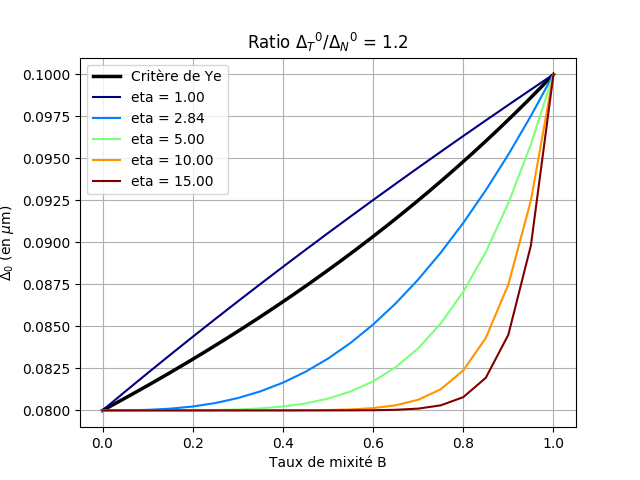
\({\mathrm{\Delta }}_{N}^{0}=0.08\mathrm{\mu }m\)

\({\mathrm{\Delta }}_{T}^{0}=0.10\mathrm{\mu }m\)

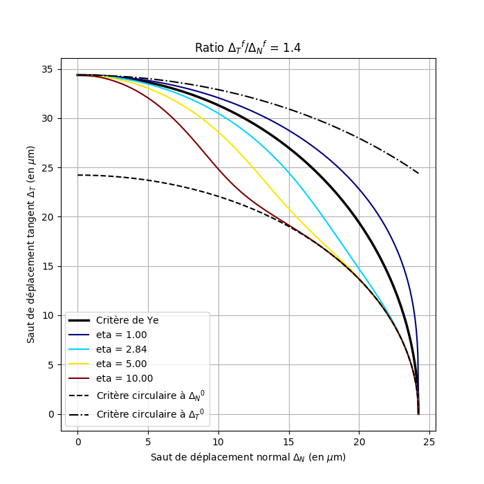
\({\mathrm{\Delta }}_{N}^{f}=24\mathrm{\mu }m\)

\({\mathrm{\Delta }}_{T}^{f}=34\mathrm{\mu }m\)

With this set of parameters, we can see that the normal and tangent properties are not extremely different (ratio 1.2 for damage initiation properties, 1.4 for propagation properties).

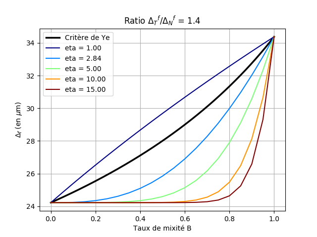
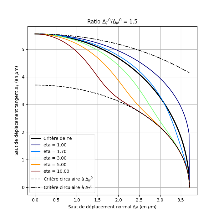
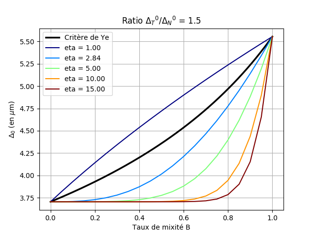
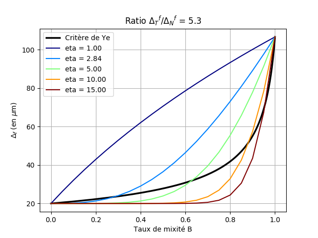
In FIGS. (a) and (b), it can be seen that the threshold surfaces of the Turon criterion may be above or below the elliptical criterion depending on the values of the power parameter \(\mathrm{\eta }\) and that the two criteria are even very similar for certain values of \(\mathrm{\eta }\). This is particularly the case for the value from the article, which was based on experimental tests, namely \(\mathrm{\eta }=2.84\). The effect of parameter \(\mathrm{\eta }\) is easier to understand in figures (c) and (d): the greater the parameter \(\mathrm{\eta }\), the longer it « takes » to pass to the tangent mode value as the mixing rate increases from 0 (pure normal mode) to 1 (pure tangent mode) to 1 (pure tangent mode). The « circular » criteria have also been represented, in dashed lines, i.e. if the normal and tangent properties are equal, which corresponds to the case of law CZM_LIN_REG.

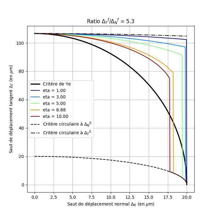
These same curves can be visualized in the figure with properties determined in the context of the experimental characterization of an interlaminar joint (between two distinct composites) that can typically be found in a wind turbine blade. The properties are not explicitly given here (the initiation and damage jumps can nevertheless be read on the curves): the important thing is that the relationship between the normal and tangent properties is more important, especially with regard to the propagation of the crack. On the figure

Since this law of behavior was initially developed to model the damage of glued joints, we did not consider cases where the normal properties are greater than the tangent properties, because it is not representative of reality: normal stress (peeling) is generally more critical for a bonded joint than shear stress.

Figure 2.2.2: Visualization of the Turon criteria (for different values of θ) and Ye with the material properties from [1]: (a) damage initiation threshold surfaces; (b) evolution of the initiation jump as a function of the mixing rate; (c) crack propagation threshold surfaces; (c) crack propagation threshold surfaces; (d) evolution of the propagation jump as a function of the mixing rate. Attention, the scales according to X and Y are different.

Figure 2.2.3: Visualization of the Turon criteria (for various values of θ) and Ye with the material properties resulting from a joint characterization campaign: (a) damage initiation threshold surfaces; (b) evolution of the initiation jump as a function of the mixing rate; (c) crack propagation threshold surfaces; (c) crack propagation threshold surfaces; (d) evolution of the propagation jump as a function of the mixing rate. Attention, the scales according to X and Y are different.

This formulation ensures a continuous transition between damage threshold surfaces, where the threshold surface associated with \(d=0\) is the damage initiation surface, and that associated with \(d=1\) the crack propagation surface.

It can be visualized in Figure, obtained with the parameter values given above and derived from [1] by the fact that the threshold surfaces (changing as a function of damage \(d\)) are well intertwined with each other as \(d\) increases and does not intersect. Thus, if the mixing of the loading changes, the mixing rate corresponding to the angle in diagram \(({\mathrm{\Delta }}_{N},{\mathrm{\Delta }}_{T})\), there will be no « self-healing » of the cohesive element (the evolution of \(d\) is very monotonic increasing), and the dissipation energy will always be positive. For a « self-healing » element, damage \(d\) could decrease with the change in mixing rate, as shown schematically in Figure.

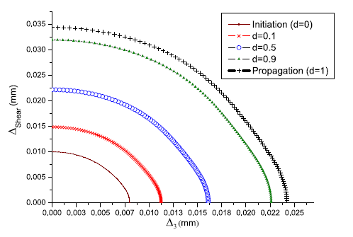
Figure 2.2.4: Surface damage threshold in travel space (with shear ≡ T and 3 ≡ N here) [1]

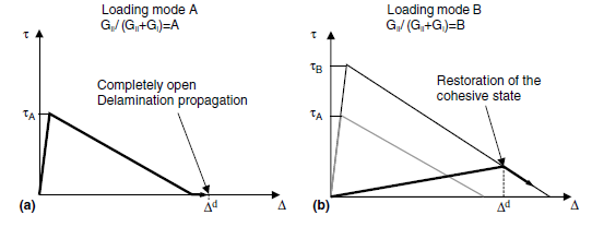
Figure 2.2.5: Example of « self-healing » of a cohesive element when the loading rate changes from A to B [1]

2.3. Tangent matrix#

The tangent matrix is necessary for the numerical implementation of the law of behavior in the context of the resolution of mechanical equations by Newton’s algorithm.

The tangent matrix is obtained by differentiating the behavior equation:

Where did we use

We define

Let’s focus on quantity

In a dissipative regime we have:

Here, we are neglecting the variation in quantities

and

depending on

, which depend on it via the mix rate. So we make the assumption that the mixed loading rate does not change too abruptly. If necessary, care should be taken to discretize the load sufficiently to satisfy this hypothesis during a calculation.

and in addition:

Where did we use

Finally, we get the tangent matrix

in a dissipative regime

in linear mode

With, we remind you:

We note that the matrix

is not defined in

. We’ll extend the function to the right at this point.

2.4. Internal variables of law CZM_TURON#

Law CZM_TURON has internal variables. From the point of view of implementing the behavior, only the first is an internal variable in the thermodynamic sense. The others are post-treatments that provide information on the condition of the joint at a given moment.

! V1: PLUS GRANDE NORME DU SAUT É QUIVALENT TOTAL (variable)