2. Internal discontinuity model

This model makes it possible to take into account the initiation and propagation of cracks in a structure for a given direction. This is based on specific finite elements called elements with internal discontinuity (from the English embedded discontinuity finite elements). The main idea is based on the introduction of a discontinuity included in the element and an internal threshold variable managing the dissipative process as well as the irreversible nature of the cracking. In addition, the displacement jump will be considered constant per element, which will facilitate numerical resolution. It is possible to adopt a static condensation technique where the calculation of the jump during minimization will be done at the elementary level.

The discontinuity element was developed in order to avoid the regulation of energy into zero (penalized adherence) of law CZM_EXP_REG developed for the joint element (see documentation [R3.06.09] for the element and [R7.02.11] for the law). In fact, this is harmful for models based on a principle of minimum energy since it leads to the cancellation of the derivative of the surface energy density at zero, that is to say the critical constraint of the model. In such a situation, the initiation of a crack occurs as soon as loading occurs, however weak it may be (note, however, that this does not prevent obtaining interesting results with such a law, as soon as the cracking path is fixed).

To take into account the discontinuity, displacements and deformations are enriched in order to ensure their compatibility.

In this part we will first present the law of behavior that governs the element with discontinuity. We will have to define a stress vector in the element that will be used during the minimization of energy. We will then detail the properties of the finite element and then the numerical resolution of the energy minimization problem.

2.1. Law of behavior of the element with discontinuity: CZM_EXP

Discontinuous elements have mixed behavior: elastic and dissipative. The total energy of the element is written as the sum of elastic energy and surface energy of type CZM. The following parts will be devoted to the presentation of this last one as well as to the constraint that derives from it.

2.1.1. Total energy in the discontinuous element

We choose the total energy \({E}_{T}\) as the sum of an elastic energy defined on the element noted \({\Omega }_{e}\) and a surface energy defined on the discontinuity of the element noted \({\Gamma }_{e}\):

(2.1)\[ {E} _ {T} (U,\ delta;\ kappa) =\ Phi (U,\ delta) +\ Psi (\ delta,\ kappa)\]

where \(\Phi\) corresponds to elastic energy. Note that this depends on the node displacement \(U\) and the displacement jump

constant (in the element) which will be seen to induce additional deformation. Surface energy \(\Psi\) depends on the displacement jump and on \(\kappa\) internal variable to treat the irreversibility of the crack.

Note: The crack path is known a priori, the normal to the discontinuity will therefore be fixed by the orientation of the elements in the mesh (see figure).

2.1.1.1. Elastic energy

To define elastic energy we will need to introduce the interpolation of the displacement field in the discontinuous element right now, however, the properties of the latter will be detailed in a section to follow (see § 2.2). In the figure, we represent the element with discontinuity noted \({\Omega }_{e}\), it is a quadrangle with four nodes with an internal discontinuity that we note \({\Gamma }_{e}\).

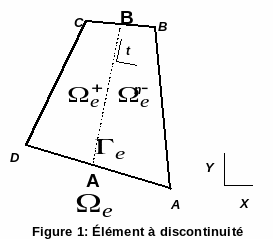
Figure 1: Discontinuous element

The interpolation of the \(u(x)\) displacement field in the discontinuity element is written as:

(2.2)\[\begin{split} u (x) =N (x)\ mathrm {.} \ left [\ begin {array} {c} {U} _ {U} _ {A}\\ {U} _ {B}\\ {U} _ {C} -\ delta\ {U} _ {D} -\ delta\ end {array} {U}} -\ delta\ end {array}\ {array}\\ {array}\ right] _ {H} _ {\ Gamma} _ {e}} -\ delta\ {U} _ {D} -\ delta\ end {array}\ {array}\ right] + {H} _ {\ Gamma} _ {e}} (x)\ mathrm {.} \ delta\end{split}\]

with \(N\) matrix of functions of classical bilinear form of type \(\mathrm{Q1}\), \({H}_{{\Gamma }_{e}}\) the Heaviside function on the discontinuity of the element \({\Gamma }_{e}\) being equal to 1 if \(x\in {\Omega }_{e}^{\text{+}}\) and 0 if \(x\in {\Omega }_{e}^{\text{-}}\). Vector \(\delta\) corresponds to the jump in movement over the discontinuity. We have \(〚u〛=\delta\) since \(N\) is a continuous function and \({H}_{{\Gamma }_{e}}=1\) is over \({\Gamma }_{e}\). In addition, the \(U\) (indexed by the vertices) correspond to the nodal movements, in fact we can write:

(2.3)\[\begin{split} \ left\ {\ begin {array} {c} {U} _ {A}\\ {U} _ {B}\\ {U} _ {C}\\ {U} _ {D}\ end {array}\ right\}\ right\} =\ left\ {array} {U} _ {B}\ {U}\ {U}\ {U}\\ {U}\ right\}\ right\}\ right\}\ right\}\ right\}\ right\}\ right\}\ right\}} =\ left\ {\ begin {U}\ right\}}\ right\}\ right\}}\ right\}\ right\}\ right\}}\ right\}\ right\}\ right\}\ right\}}\ right\}\ right\}\ right\}}\ delta -\ delta\\ {U} _ {D} +\ delta -\ delta\ end {array}\ right\}\end{split}\]

From the approximate field () we can define the associated deformation on the element outside of the discontinuity:

(2.4)\[\begin{split} \ epsilon\ mathrm {=} {\ mathrm {\nabla}} ^ {\ text {s}} N (x)\ mathrm {.} \ left\ {\ begin {array} {c} {U} {U} _ {A}\\ {U} _ {B}\\ {U} _ {C}\ mathrm {-}\ delta\\ {U} _ {D} _ {D}\ mathrm {-}\ mathrm {-} _ {-}\ mathrm {-}} _ {\ underset {-}\}} {{\ mathrm {\nabla}}} ^ {\ text {s}} {H} _ {{\ Gamma} _ {e}} (x)}}}\ mathrm {\ cdot}\ delta\end{split}\]

\({\nabla }^{\text{s}}\) refers to the symmetrized gradient. We can rewrite () in synthetic form:

(2.5)\[ \ epsilon =B\ mathrm {.} U-D\ mathrm {.} \ delta\]

where \(B\) is the matrix of the symmetrized gradients of the shape functions, \(U={({U}_{A},{U}_{B},{U}_{C},{U}_{D})}^{T}\) and \(D\mathrm{.}\delta =B{(\mathrm{0,}\mathrm{0,}\delta ,\delta )}^{T}\). In the expression () we distinguish one part of the deformation linked to the movements \(B\mathrm{.}U\) and another part \(-D\mathrm{.}\delta\) linked to the jump. The constraint for an elastic law of behavior is written as:

\[\]

: label: eq-21

sigmamathrm {=} Emathrm {.} Epsilon

With \(E\) the elasticity tensor. The elastic energy in the element is therefore defined by:

(2.6)\[ \ Phi (U,\ delta) =\ frac {1} {2}\ mathrm {.} {\ int} _ {{\ omega} _ {e}}} {(B\ mathrm {.} U-D\ mathrm {.} \ delta)} ^ {T}\ mathrm {.} E\ mathrm {.} (B\ mathrm {.} U-D\ mathrm {.} \ delta)\ mathrm {.} d\ Omega\]

2.1.1.2. Surface energy

As we presented in the theoretical model (see § 1), we choose a surface energy depending on the norm of the displacement jump \(\parallel \delta \parallel\), on \(\kappa\) positive internal variable (its initial value \({\kappa }_{0}\) is zero) and on the orientation of the crack (only for the contact condition). We take:

(2.7)\[ \ Psi (\ delta,\ kappa) =H (\ parallel\ delta\ parallel -\ kappa)\ mathrm {.} {\ Psi} _ {\ mathrm {dis}} (\ parallel\ delta\ parallel) +\ left [1-H (\ parallel\ delta\ parallel -\ kappa)\ right]\ mathrm {.} {\ Psi} _ {\ mathrm {lin}}} (\ parallel\ delta\ parallel,\ kappa) + {I} _ {{↓} ^ {\ text {+}}}} (\ delta\ cdot n)\]

The indicator function \({I}_{{ℝ}^{\text{+}}}\) makes it possible to take into account the condition of non-interpenetration of the lips of the crack:

(2.8)\[\begin{split} {I} _ {{328} ^ {\ text {+}}}} ({\ delta} _ {n}) =\ {\ begin {array} {cc} +\ infty &\ text {si}\ delta\ cdot n<0\\ cdot n<0\\ cdot n<0\\ cdot n<0\\ cdot n<0\\ cdot n<0\\ cdot n<0\\ cdot n<0\\ 0&\ text {si}\ delta\ cdot n\ ge 0\ end {array}\end{split}\]

Depending on the threshold value, the surface energy will be worth \({\Psi }_{\mathrm{dis}}\) or \({\Psi }_{\mathrm{lin}}\) (plus the indicator function). In the first case we will speak of a dissipative regime, in the second case of linear regime. We can write the two energies in the form:

(2.9)\[ {\ Psi} _ {\ mathrm {dis}}} (\ parallel\ delta\ parallel) = {\ int} _ {\ Gamma} _ {\ psi}} {\ psi} _ {\ mathrm {dis}}} (\ parallel\ delta\ parallel)\ mathrm {.} d\ Gamma\]

with \({\psi }_{\mathrm{dis}}\) and \({\psi }_{\mathrm{lin}}\) surface energy densities. Let us present the values of these densities in detail.

Surface energy density in linear status

In the case where an existing crack evolves (opening or reclosing) without dissipating energy i.e. \(\parallel \delta \parallel <\kappa\), the element will be in a linear phase (charge or discharge). We therefore choose an energy density that is a quadratic function of the jump norm:

(2.10)\[ {\ Psi} _ {\ mathrm {lin}} (\ parallel\ delta\ parallel,\ kappa) =\ frac {1} {2}\ mathrm {.} P (\ kappa)\ mathrm {.} {\ parallel\ delta\ parallel} ^ {2} + {C} _ {0}\]

where \(P(\kappa )\mathrm{=}\frac{{\sigma }_{c}}{\kappa }\mathrm{.}\mathrm{exp}(\mathrm{-}\frac{{\sigma }_{c}}{{G}_{c}}\mathrm{.}\kappa )\) is chosen in order to ensure the continuity of the derivative of \(\Psi\) in \(\kappa\) (i.e. the continuity of the stress in the element from one regime to another) and the constant \({C}_{0}\) to ensure the continuity of \(\Psi\) in \(\kappa\).

Dissipative energy density

Inspired by Barenblatt [1]”s idea of taking into account the process of breaking inter-atomic bonds, we assume that the surface energy is zero at zero and increases towards Griffith energy when the value of the jump becomes important in front of the characteristic length of the atomic scale. Moreover, relying on the shape of the inter-atomic potentials, an increasing concave energy with a convex derivative is chosen. In particular, we know that concavity plays an essential role in dimension 1 to limit the number of cracks (see Charlotte et al. [2]). Thus, in the case where \(\parallel \delta \parallel <\kappa\), a surface energy density of the following form is chosen, illustrated in the figure:

\[\]

: label: eq-27

{Psi} _ {mathrm {dis}}} (paralleldeltaparallel) = {G} _ {mathrm {c.}} left [1-mathrm {exp} (-frac {{sigma} _ {sigma} _ {c}}}mathrm {.}} paralleldeltaparallel)right]

\({G}_{c}\) represents the critical energy release rate (or toughness) of the material and \({\sigma }_{c}={\Psi }_{\mathrm{rev}}^{\text{'}}(0)\) represents the critical stress.

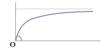
Figure 2: Surface energy density as a function of the jump norm

2.1.2. Stress vector in the discontinuous element

Let \(\overrightarrow{\sigma }=({\sigma }_{n},{\sigma }_{t})\) be the stress vector in the element. When the element \((\kappa =0)\) is healthy, the surface energy is zero. The stress vector is defined from the stress tensor of the law of elastic behavior and from the normal to the discontinuity line:

(2.11)\[ \ overrightarrow {\ sigma} =\ sigma\ cdot n\]

We will see later (see § 2.3.1.1 on the priming criterion) that the jump remains zero as long as the norm of the stress vector does not reach the critical constraint \({\sigma }_{c}\). On the other hand, if the threshold \(\kappa\) is not zero, the stress vector in the element is given by the derivative of the surface energy density with respect to the jump (the stress vector remains equal to \(\sigma \cdot n\) since the element ensures the continuity of the normal stress, see § 2.2.2).

2.1.2.1. Linear regime

In linear mode (\(\parallel \delta \parallel <\kappa\)), the stress vector is equal to:

(2.12)\[ \ overrightarrow {\ sigma} =\ frac {\ partial {\ Psi} _ {\ mathrm {lin}}} {\ partial\ delta} =P (\ kappa)\ mathrm {.} \ delta\]

And its derivative with respect to the jump:

\[\]

: label: eq-30

frac {partialoverrightarrow {sigma}} {partialdelta} =mathrm {Id}mathrm {.} P (kappa)

2.1.2.2. Dissipative regime

In the dissipative regime (\(\parallel \delta \parallel >\kappa\)), the stress vector is equal to:

\[\]

: label: eq-31

overrightarrow {sigma}mathrm {=}frac {mathrm {partial} {psi} _ {mathit {dis}}}} {mathrm {partial}delta}delta}delta}mathrm {=} {sigma} _ {c}mathrm {.} frac {delta} {mathrm {parallel}deltamathrm {parallel}}mathrm {.} mathrm {exp} (mathrm {-}frac {{sigma} _ {sigma}} {{G} _ {c}}}mathrm {.}} mathrm {parallel}deltamathrm {parallel})

And its derivative with respect to the jump:

(2.13)\[ \ frac {\ partial\ overrightarrow {\ sigma}} {\ partial\ delta} = {\ sigma} _ {c}\ mathrm {.} \ left [\ frac {\ mathrm {Id}} {\ parallel\ delta\ parallel} -\ frac {\ delta} {\ parallel\ delta\ parallel}\ otimes\ frac {\ delta} {\ frac {\ delta} {\ parallel\ delta} {\ parallel\ delta\ parallel}\ mathrm {.} (\ frac {{\ sigma} _ {c}}} {{G}} _ {c}} +\ frac {1} {\ parallel\ delta\ parallel})\ right]\ mathrm {.} \ mathrm {exp} (-\ frac {{\ sigma} _ {\ sigma} _ {\ sigma}} _ {c}}\ mathrm {.}} \ parallel\ delta\ parallel)\]

2.1.2.3. Graphic illustration

The figure shows the evolution of the norm of the stress vector in the element as a function of the norm of the jump. The arrows represent the possible evolutions of the stress vector depending on the case (healthy element, linear regime or dissipative regime).

Figure 3: Norm of the stress vector as a function of the norm of the jump

To the jump threshold \(\kappa\) corresponds to a constraint threshold that is noted \(R(\kappa )\). The latter will determine at what level of stress the crack will dissipate energy. This threshold will change with the opening of the crack, it depends on

and is defined by:

(2.14)\[ R (\ kappa)\ mathrm {=} {\ sigma} _ {c}\ mathrm {.} \ mathrm {exp} (\ mathrm {-}\ frac {{\ sigma} _ {\ sigma}} {{G} _ {c}}}\ mathrm {.}} \ kappa)\]

Note that when \(\kappa =0\) this threshold corresponds to the priming criterion that we will present in § 2.3.1.1.

2.2. Properties of the discontinuous element

The discontinuous element is a quadrangle with four nodes with an internal displacement jump. A first part will be devoted to the geometric description of the element as well as to the presentation of a configuration based on the reference element. Next, we will see that the element ensures the continuity of the normal stress through the displacement jump. Then, we will show the uniqueness of the jump movement as long as the size of the element is small enough. Finally, we will see that choosing a constant jump introduces a parasitic surface energy that tends to zero when we refine the mesh.

2.2.1. Element geometry and parameterization

2.2.1.1. Geometry

Let \((X,Y)\) be the Cartesian base constituting a global coordinate system of \({ℝ}^{2}\). The discontinuity element, noted \({\Omega }_{e}\), is a finite quadrangle element with four nodes. It consists of an elastic region and a discontinuity \({\Gamma }_{e}\) passing through the center of the element (segment passing through the midpoints of the sides \([\mathrm{AD}]\) and \([\mathrm{BC}]\)) and of length \(l\) (see figure).

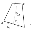
Figure 4: Discontinuous element The orientation of the discontinuity defines a coordinate system that is local to element \((n,t)\). The corresponding reference element is a \(\stackrel{ˆ}{{\Omega }_{e}}\) square defined by the \([-\mathrm{1,1}]\times [-\mathrm{1,1}]\) domain (see figure). Each of the elements has four Gauss points. Those in the reference element have coordinates \((\pm \sqrt{(3)}/3,\pm \sqrt{(3)}/3)\). Let’s note \({\omega }_{g}\) and \(\stackrel{ˆ}{{\omega }_{g}}\) the weights of the Gauss points respectively in the real configuration and in the reference configuration. Finally, remember that the approximation of the displacement field in the element was presented in part§ 2.1.1.1.

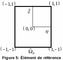
Figure 5: Reference element

2.2.1.2. Parameterization

Figure 6: Parameterization of the discontinuity element Let \(T\) be the geometric transformation that associates a point \((\eta ,\xi )\) of the reference element at a point \((x,y)\) of the discontinuity element at a point of the discontinuity element. Let’s try to set the position of any point \(M\) of the discontinuous element by \((\eta ,\xi )\) its coordinates in the coordinate system of the reference element.

Let \(P\), \(Q\) and \(M\) be the points (see figure) such as:

(2.15)\[\begin{split} \ {\ begin {array} {c}\ overrightarrow {\ mathrm {AP}} =\ frac {1} {2}\ mathrm {.} (1+\ xi)\ mathrm {.} \ overrightarrow {\ mathrm {AB}}}\\\ overrightarrow {\ mathrm {DQ}} =\ frac {1} {2}\ mathrm {.}} (1+\ xi)\ mathrm {.} (1+\ xi)\ mathrm {.} \ overrightarrow {\ mathrm {DC}}}\\\ overrightarrow {\ mathrm {PM}} =\ frac {1} {2}\ mathrm {.} (1-\ eta)\ mathrm {.} (1-\ eta)\ mathrm {.} \ overrightarrow {\ mathrm {PQ}}}\ end {array}\end{split}\]

Using the sum of the vectors, we have:

(2.16)\[ \ overrightarrow {\ mathrm {AM}} =\ overrightarrow {\ mathrm {AP}} +\ overrightarrow {\ mathrm {PM}}} =\ frac {1} {2} {2}\ mathrm {2}}\ mathrm {.} (1+\ xi)\ mathrm {.} \ overrightarrow {\ mathrm {AB}}} +\ frac {1} {2}\ mathrm {.} (1-\ eta)\ mathrm {.} \ overrightarrow {\ mathrm {PQ}}\]

We rewrite vector \(\overrightarrow{\mathrm{PQ}}\):

(2.17)\[ \ overrightarrow {\ mathrm {PQ}} =\ overrightarrow {\ mathrm {PA}} +\ overrightarrow {\ mathrm {AD}}} +\ overrightarrow {\ overrightarrow {\ mathrm {DQ}}\]

By expanding with expressions from ():

(2.18)\[ \ overrightarrow {\ mathrm {PQ}} =\ frac {1} {2}\ mathrm {.} (1+\ xi)\ mathrm {.} \ overrightarrow {\ mathrm {BA}}} +\ overrightarrow {\ mathrm {AD}} +\ frac {1} {2}\ mathrm {.} (1+\ xi)\ mathrm {.} (1+\ xi)\ mathrm {.} \ overrightarrow {\ mathrm {DC}}\]

By grouping the terms together, we finally get:

(2.19)\[ \ overrightarrow {\ mathrm {AM}} =\ frac {1+\ eta} {2}\ mathrm {.} \ frac {1+\ xi} {2}\ mathrm {.} \ overrightarrow {\ mathrm {AB}}} +\ frac {1-\ eta} {2}\ mathrm {.} \ overrightarrow {\ mathrm {AD}}} +\ frac {1-\ eta} {2}\ mathrm {.} \ frac {1+\ xi} {2}\ mathrm {.} \ overrightarrow {\ mathrm {DC}}\]

And so:

(2.20)\[\begin{split} dM=\ left\ {\ begin {array} {c} {c}\ mathrm {xx}\\ mathrm {dy}\ end {array}\ right\} =\ frac {N (\ xi)} {2} {2}\ mathrm {.} d\ mathrm {.} d\ xi\end{split}\]

With the two vectors of the coordinate system on the discontinuity:

(2.21)\[\begin{split} \ {\ begin {array} {c} N (\ xi) =\ left\ {\ begin {array} {c} {N} _ {x}\ {N} _ {y}\ end {array}\\ right\} =\ right\} =\ frac {(1+\ xi)} {2}\ mathrm {.} \ overrightarrow {\ mathrm {AB}}} -\ frac {(1-\ xi)} {2}\ mathrm {.} \ overrightarrow {\ mathrm {DC}}} -\ overrightarrow {\ mathrm {AD}}\\ T (\ eta) =\ left\ {\ begin {array} {c} {T} {T} _ {x} _ {x}\\ {T}\\ {T} _ {y}\ end {array}\ right\}} =\ frac {(1+\ eta)} {2}\ mathrm {.} \ overrightarrow {\ mathrm {AB}}} +\ frac {(1-\ eta)} {2}\ mathrm {.} \ overrightarrow {\ mathrm {DC}}}\ end {array}\end{split}\]

We then have the configuration:

(2.22)\[\begin{split} \ left\ {\ begin {array} {c}\ mathrm {xx}\\ mathrm {dy}\ end {array}\ right\} =\ left [J\ right]\ mathrm {.} =\ left [J\ right]\ mathrm {.} \ left\ {\ begin {array} {c} {c} d\ eta\\ d\ xi\ end {array}\ right\}\end{split}\]

Where \(\left[J\right]\) is the Jacobian matrix for the transformation:

(2.23)\[\begin{split} \ left [J\ right] =\ frac {1} {1} {2}\ mathrm {.} \ left [\ begin {array} {cc} {N} {N} _ {n} _ {x} _ {x}\\ {N} _ {y} & {T} _ {y}\ end {array}\ right]\end{split}\]

Note: Since the discontinuity is located at the center of the element, we can define the vectors of the coordinate system local to it as well as its length from the vector \(T\) in \(\eta =0\):

(2.24)\[\begin{split} \ {\ begin {array} {c} n= {R} _ {-\ pi /2} T (0)/\ parallel T (0)\ parallel\\ t=T (0)/\ parallel T (0)\ parallel (0)\ parallel\\ n=\ parallel\ l=\ parallel T (0)\ parallel\ end {array}\end{split}\]

2.2.2. Continuity of normal stress

Based on the previous setting, we show in [6] how the discontinuous element ensures the continuity of the normal stress through the displacement jump when the stress is homogeneous in the element. In other words, we show that the stress vector \(\overrightarrow{\sigma }={\psi }^{\text{'}}(\delta )\) of the law of behavior CZM_EXP (see § 2.1.2) is equal to the normal stress in the element \(\sigma \mathrm{.}n\).

2.2.3. Condition of existence and uniqueness of the jump in the element

From a numerical point of view, it is important to put yourself in a situation where the search for the jump in the element leads to a unique solution. In other words it is necessary for the solution of the minimization problem () to have a single solution to \(U\) and \(\kappa\) fixed.

(2.25)\[ \ underset {\ delta\ in {↓} ^ {2}}} {\ text {min}} {E} _ {T} (U,\ delta,\ kappa)\]

In [6] we show that the existence and the uniqueness of the jump are ensured as soon as the following condition, relating to the geometry as well as to the material parameters of the element, is ensured:

(2.26)\[ \ frac {\ mu} {16}\ mathrm {.} \ sum _ {g} (\ frac {1} {{\ omega} _ {g}}\ mathrm {.} \ underset {{\ eta} _ {g}}} {\ text {min}} {\ text {min}} {\ parallel T ({\ eta} _ {g})\ parallel} ^ {2}) >l\ mathrm {.} \ frac {{\ sigma} _ {c} ^ {2}} {{G} _ {c}}\]

Note: In the particular case where the discontinuous element is rectangular, the weights of the Gauss points are equal to a quarter of the area of the element. Also, the length of the element is equal to the length of the \(l\) discontinuity. If we write \(e\) the width of the element, we have \(g\) for everything:

(2.27)\[ {\ omega} _ {g} =\ frac {l\ mathrm {.} e} {4}\]

Plus \(\parallel T\parallel =l\) on each Gauss point, so the condition of uniqueness becomes a condition on the width of the element:

(2.28)\[ e<\ mu\ mathrm {.} \ frac {{G} _ {c}}} {{\ sigma} _ {c} ^ {2}}\]

It is this last condition that ensures the uniqueness of the jump for the elements with discontinuity in Code_Aster. It is therefore necessary to handle these with care when they are not rectangular in shape and to ensure that the condition given by () is true.

2.2.4. Parasitic energy

The constant jump in the discontinuous element leads to the introduction of parasitic energy at the interface between two adjacent elements. We show in [6] that this energy tends to zero when we refine the mesh.

2.3. Minimization of total energy

By adopting the principle of energy minimization, the aim of this part is to present the calculation of the displacement jump in discontinuous elements as well as that of the displacement field. The total energy (see § 2.1.1) is not convex with respect to the \((U,\delta )\) couple. The search for a global minimum for such a functional is not possible with the numerical method that we will use. Moreover, under imposed force, the total energy not being bounded lower, the global minimum does not exist. These two arguments lead us to make the choice to look for a local minimum. The total energy minimization problem is written as:

(2.29)\[ \ text {Search} ({U} ^ {\ text {*}}}, {\ text {*}}}, {\ delta} ^ {\ text {*}})\ text {local total energy minimum} {E} _ {T} (U,\ delta,\ kappa)\]

In a first section (§ 2.3.1) we will try to calculate \({\delta }^{\text{*}}\) local minimum of the total energy at \(U\) fixed:

(2.30)\[ {\ delta} ^ {\ text {*}}} (U) =\ underset {\ delta} {\ text {argmin}} {E} _ {T} (U,\ delta,\ kappa)\]

In the second section (§ 2.3.2), we will content ourselves with looking for a condition necessary for \({U}^{\text{*}}\) to be the local minimum of the total energy with \(\delta ={\delta }^{\text{*}}(U)\):

\[\]

: label: eq-50

{U} ^ {text {*}}} =underset {U} {text {argmin}} {E} _ {T} (U, {delta} ^ {text {*}}} (U),kappa)

This second step amounts to solving the equilibrium equations taking into account any work, external forces and displacements imposed on the structure.

Note: The numerical treatment of the indicator \({I}_{{ℝ}^{\text{+}}}(\delta \cdot n)\), representing the condition of non-interpenetration of the lips of the crack, will be performed by adding the \(\delta \cdot n\ge 0\) constraint to the minimization problem.

2.3.1. Minimization of total energy compared to jumping

The purpose of this section is to calculate the movement jumps, on each of the discontinuous elements of a mesh, which minimize the total energy. If we index the elements with discontinuity by \(i\) and we note \({\delta }_{i}\) the jumps in movement on each of these elements, the minimization problem is written as:

(2.31)\[ \ mathrm {Search}\ mathrm {les} {\ delta} _ {i} _ {i}\ text {local minima of total energy, solutions of}\ underset {{\ delta} _ {i}, {\ delta} _ {i} _ {i} _ {i} _ {i} _ {i} _ {i} _ {i} (U, {\ delta} _ {i} _ {i} _ {i} _ {i} _ {i} _ {i} _ {i} _ {i} _ {i} _ {i} _ {i} _ {i} _ {i} _ {i} _ {i} _ {i} _ {i} _ {i} _ {i} _ {i} _ {i} _ {i} _ {i} _ {i} _ {i}},\ kappa)\]

Two important points will make it possible to significantly simplify the problem. First of all, the choice of an independent displacement jump from one element to another makes it possible to minimize the total energy compared to the jump at an elementary level (static condensation technique). We have the following equality:

\[\]

: label: eq-52

underset {{delta} _ {i}, {delta} _ {i} _ {i}cdot nge 0} {text {min}}}sum _ {E} _ {T} (U, {delta} _ {i} _ {i},kappa) =sum _ {i},kappa) =sum _ {i}cappa) =sum _ {i}}cpa dot nge 0} {text {min}}} {E} _ {T} (U, {delta} _ {i},kappa)

Moreover, we saw in § 2.2.3 that, for sufficiently small elements, the displacement jump is unique. Thus, the problem comes down to a search for a global minimum on each element:

(2.32)\[ \ text {On each item search}\ delta\ in S\ text {global minimum of} {E} _ {T} (U, {\ delta} _ {i},\ kappa)\]

with \(S\) the set of eligible jumps:

(2.33)\[ S=\ {s/s\ text {element-wise constant and} s\ cdot n\ ge 0\}\]

The equilibrium condition called the first-order optimality condition becomes necessary and sufficient to determine the solution of the problem. It is written in the form:

(2.34)\[ {E} _ {T} (U,\ delta,\ kappa)\ le {E} _ {T} (U,\ delta +h\ phi,\ kappa)\]

For any constant \(\phi\) per element and for \(h\) small enough so that \(\delta +h\phi \in S\). Passing to the limit when \(h\) approaches zero, it becomes a condition on the directional derivative:

(2.35)\[ \ underset {h\ to 0} {\ mathrm {lim}}\ frac {1} {h}\ mathrm {.} ({E} _ {T} (U,\ delta +h\ phi,\ kappa) - {E} _ {T} (U,\ delta,\ kappa))\ ge 0\]

For any constant \(\phi\) per element such as \(\delta +h\phi \in S\). In general, the directional derivative is a positively homogeneous function of degree one in \(\phi\).

Next, we will present the calculation of the jump displacement on an element, based on the optimality condition. We will begin by identifying a necessary and sufficient condition, which will be called the priming criterion, for the zero jump to be a solution to the problem. Then we will detail the calculation of the jump after priming, for the two types of behavior of the element: linear and dissipative.

2.3.1.1. Priming criterion

In this part we will try to determine under which condition the zero displacement jump is a solution to the problem (). Note that the choice to make the surface energy depend on the jump norm implies that the total energy does not admit a zero derivative. Therefore the derivative of the energy in the \(\phi\) direction will not be a linear function but a positively homogeneous function of degree one in \(\phi\). Using the definition of total energy (see § 2.1.1) when the element is healthy (i.e. when \(\kappa =0\)), we calculate its derivative in the \(\phi\) direction at zero:

(2.36)\[ \ underset {h\ to 0} {\ mathrm {lim}}\ frac {1} {h}\ mathrm {.} ({E} _ {T} (U, h\ phi,\ kappa) - {E} _ {T} (U,\ mathrm {0,}\ kappa)) =-\ sum _ {g} {g} {g} {g}\ mathrm {.} {\ phi} ^ {t}\ mathrm {.} {D} _ {g} ^ {t}\ mathrm {.} E\ mathrm {.} {B} _ {g}\ mathrm {.} u+l\ mathrm {.} {\ sigma} _ {c}\ mathrm {.} \ parallel\ phi\ parallel\]

The optimality condition () therefore leads to inequality:

(2.37)\[ -\ sum _ {g} {\ omega} _ {g}\ mathrm {.} {\ phi} ^ {t}\ mathrm {.} {D} _ {g} ^ {t}\ mathrm {.} E\ mathrm {.} {B} _ {g}\ mathrm {.} u+l\ mathrm {.} {\ sigma} _ {c}\ mathrm {.} \ parallel\ phi\ parallel\ ge 0\]

For everything \(\phi \in S\). However, to show the continuity of the normal stress (see [6]), we saw that:

(2.38)\[ \ sum _ {g} {\ omega} _ {g}\ mathrm {.} {D} _ {g} ^ {t}\ mathrm {.} E\ mathrm {.} {B} _ {g}\ mathrm {.} U=\ mathrm {l.} \ overrightarrow {\ sigma}\]

Also \(\phi\) is constant on the element, so () becomes:

(2.39)\[ -\ overrightarrow {\ sigma}\ cdot\ phi + {\ sigma} _ {c}\ mathrm {.} \ parallel\ phi\ parallel\ ge 0\]

By setting \(\{\begin{array}{c}{\phi }_{n}=\rho \mathrm{.}\mathrm{cos}\theta \\ {\phi }_{t}=\rho \mathrm{.}\mathrm{sin}\theta \end{array}\) with \(\rho >0\) and \(\frac{-\pi }{2}\le \theta \le \frac{\pi }{2}\) so that \({\phi }_{n}\ge 0\), and using the definition \(\overrightarrow{\sigma }=({\sigma }_{n},{\sigma }_{t})\), we get the condition:

(2.40)\[ {\ sigma} _ {n}\ mathrm {.} \ mathrm {cos}\ theta + {\ sigma} _ {t}\ mathrm {.} \ mathrm {sin}\ theta\ le {\ sigma} _ {\ sigma} _ {c} _ {c}\ forall\ theta\ in\ left [-\ frac {\ pi} {2} {2}\ left]\]

A study of function \(f(\theta )={\sigma }_{n}\mathrm{.}\mathrm{cos}\theta +{\sigma }_{t}\mathrm{.}\mathrm{sin}\theta\) gives:

\[\]

: label: eq-62

underset {-frac {pi} {2}lethetalethetalefrac {pi} {2}} {text {sup}} f (theta) =sqrt {text {}} {text {}}} <} {sigma} _ {n} {text {> _ {text {text {} {}} {text {text {pi}} {text {pi}}} f (theta) =sqrt {text {} {} {}} =sqrt {text {} {} {}} =sqrt {text {} {}} {text {text {}} {text {} {}}

With the definition of the positive part of a quantity \(\text{<}\mathrm{.}{\text{>}}_{\text{+}}=\mathrm{max}(\mathrm{.}\mathrm{,0})\). The inequality () therefore leads to the following constraint priming criterion:

(2.41)\[ \ sqrt {\ text {<} {\ sigma} _ {n} {\ text {>}} _ {\ text {+}}} ^ {2} + {\ sigma} _ {t} ^ {2}}}\ the {\ sigma} _ {c}\]

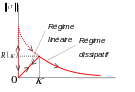
This criterion is represented in plane \(({\sigma }_{n},{\sigma }_{t})\) in the figure.

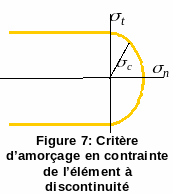
Figure 7: Criteria for initiating the stress of the discontinuity element

Remarks: This is the case where the orientation of the discontinuity \(n\) is fixed (by the mesh). This explains why we get a condition on the stress vector and not on the main components of the stress.

2.3.1.2. Jump calculation

Let’s try to solve the minimization problem in the case where the jump is not zero. In this case, the directional derivative is a linear function of \(\phi\), the optimality condition () is written as:

(2.42)\[ \ underset {h\ to 0} {\ mathrm {lim}}\ frac {1} {h}\ mathrm {.} ({E} _ {T} (U,\ delta +h\ phi,\ kappa) - {E} _ {T} (U,\ delta,\ kappa)) =\ frac {\ partial {E} _ {E} _ {T} _ {T}} {\ partial\ delta}\ cdot\ phi\ ge 0\]

For any constant \(\phi\) per element such as \(\delta +h\phi \in S\). By playing on the admissible directions, the conditions are deduced:

(2.43)\[\begin{split} \ {\ begin {array} {ccc}\ frac {\ partial {E} _ {T}} {\ partial {\ delta} _ {n}}}\ mathrm {.} {\ phi} _ {n}\ ge 0&\ forall {\ phi} _ {n}\ ge 0&\ text {\ delta} _ {n} =0\\\ frac {\ partial {E} _ {E} _ {T}}} {\ partial {\ phi}} {\ phi} _ {n}}\ mathrm {.} {\ phi} _ {n} =0&\ forall {\ phi} _ {\ phi} _ {n} _ {n} &\ text {\ delta} _ {n} >0\\ frac {\ partial {E} _ {T}} {\ forall {\ phi}} _ {\ phi} _ {n}} >0\\\ frac {\ partial {E} _ {T}}\ mathrm {.}} {\ phi} _ {t} =0&\ forall {\ phi} _ {t} &\ end {array}\end{split}\]

Moreover, by approaching the integral by a discrete sum on the Gauss points, the derivative of the total energy in the \(\phi\) direction is written:

(2.44)\[ \ frac {\ mathrm {\ partial} {E} {E} _ {T}} {\ mathrm {\ partial}\ delta}\ mathrm {\ cdot}\ phi\ mathrm {=}\ mathrm {-}\ mathrm {-}\ mathrm {-}\ mathrm {-}\ mathrm {-}\ mathrm {-}\ mathrm {-}\ mathrm {-}\ mathrm {-}\ mathrm {-}\ mathrm {-}\ mathrm {-}\ mathrm {-}\ mathrm {-}\ mathrm {-}\ mathrm {-}\ mathrm {\ phi} ^ {t}\ mathrm {.} {D} _ {g} ^ {t}\ mathrm {.} E\ mathrm {.} ({B} _ {g}\ mathrm {.} U\ mathrm {.} U\ mathrm {-} {D} _ {g}\ delta)\ mathrm {.} \ phi +l\ mathrm {.} \ frac {\ mathrm {\ partial}\ psi} {\ mathrm {\ partial}\ delta}\ mathrm {\ cdot}\ phi\]

With \(\psi\) the surface energy density, equal to \({\psi }_{\mathrm{lin}}\) in linear regime and to \({\psi }_{\mathrm{dis}}\) in dissipative regime. To simplify the notations \(S\) is defined as follows:

(2.45)\[ S\ mathrm {=}\ left\ {\ begin {array} {c} {array} {c} {c} {s} _ {t}\ end {array}\ right\}\ mathrm {=}\ mathrm {=}\ mathrm {-}\ mathrm {-}\ mathrm {-}}\ mathrm {-}\ mathrm {-}\ mathrm {-}\ mathrm {-}\ mathrm {-}\ mathrm {-}\ mathrm {-}\ mathrm {-}\ mathrm {-}\ mathrm {-}\ mathrm {-}\ mathrm {-}\ mathrm {-} { {D} _ {g} ^ {t}\ mathrm {.} E\ mathrm {.} {B} _ {g}\ mathrm {.} U\]

and \(Q\):

(2.46)\[\begin{split} Q=\ left [\ begin {array} {cc} {Q} {Q} _ {\ mathrm {nn}} _ {\ mathrm {nt}}\\ {Q} _ {\ mathrm {nt}}} & {Q}} & {Q}} & {Q}} _ {Q} _ {Q} _ {\ mathrm {tt}}} _ {\ mathrm {tt}}}\ end {array}\ right] =-\ sum _ {g} {omega}} _ {g}\ mathrm {nt}}} & {Q} {Q}} _ {\ mathrm {nt}}} & {Q} {Q}} _ {\ mathrm {nt}}} & {Q}} thrm {.} {D} _ {g} ^ {t}\ mathrm {.} E\ mathrm {.} {D} _ {g}\end{split}\]

So we have the simplified writing of ():

(2.47)\[ \ frac {\ partial {E} _ {T}}} {\ partial\ delta}\ cdot\ phi =( S+Q\ mathrm {.} \ delta)\ cdot\ phi +l\ mathrm {.} \ frac {\ partial\ psi} {\ partial\ delta}\ cdot\ phi\]

Now let’s try to calculate the jump displacement from the conditions using the derivative of energy written in the form (). We will distinguish the calculation in the linear regime from that in the dissipative regime and for each of them we will distinguish the case where the normal jump is zero from that where it is not.

Linear jump calculation

In linear regime, the surface energy density is given by:

(2.48)\[ \ psi = {\ psi} _ {\ mathrm {lin}} =\ frac {1} {2}\ mathrm {.} P (\ kappa)\ mathrm {.} \ delta\ cdot\ delta\]

The derivative of the total energy with respect to the jump () becomes:

\[\]

: label: eq-71

frac {partial {E} _ {T}}} {partialdelta}cdotphi =( S+Qmathrm {.} delta)cdotphi +lmathrm {.} P (kappa)mathrm {.} deltacdotphi

In the case of a zero normal jump \((\mathrm{0,}{\delta }_{t})\), the optimality conditions () lead to:

(2.49)\[\begin{split} \ {\ begin {array} {c} {S} {S} _ {n} + {Q} _ {\ mathrm {nt}}\ mathrm {.} {\ delta} _ {t}\ ge 0\\ {\ delta} _ {\ delta} _ {t} =-\ frac {{S} _ {t}} {{Q} _ {t} +l\ mathrm {.} +l\ mathrm {.} +l\ mathrm {.}.} + l\ mathrm {.}.} P (\ kappa)}\ end {array}\end{split}\]

The tangent jump is given explicitly by the second condition. The first requires that the normal stress in the element be negative or zero. If that were not the case, there would necessarily be a normal jump. In other words, the jump in the element will be zero as soon as the element is put into compression. This reflects the consideration of the non-interpenetration of the lips of the crack.

In the case of a strictly positive normal jump \(({\delta }_{n}>\mathrm{0,}{\delta }_{t})\), the optimality conditions () directly give the displacement jump:

(2.50)\[ \ delta =- {(Q+\ mathrm {Id}\ mathrm {Id}\ mathrm {.} l\ mathrm {.} P (\ kappa))} ^ {-1}\ mathrm {Id}\ mathrm {.} s\]

In a linear regime the internal variable \(\kappa\) does not change.

Calculation of the jump in the dissipative regime

Under the dissipative regime, the surface energy density is given by:

(2.51)\[ \ psi = {\ psi} _ {\ mathrm {dis}} = {G} _ {c}\ mathrm {.} \ left [1-\ mathrm {exp} (-\ frac {{\ sigma} _ {\ sigma} _ {c}}}\ mathrm {.}} \ parallel\ delta\ parallel)\ right]\]

The derivative of the total energy with respect to the jump () becomes:

(2.52)\[ \ frac {\ partial {E} _ {T}}} {\ partial\ delta}\ cdot\ phi =( S+Q\ mathrm {.} \ delta)\ cdot\ phi +l\ mathrm {.} {\ sigma} _ {c}\ mathrm {.} \ frac {\ delta\ cdot\ phi} {\ parallel\ delta\ parallel}\ mathrm {.} \ mathrm {exp} (-\ frac {{\ sigma} _ {\ sigma} _ {\ sigma}} _ {c}}\ mathrm {.}} \ parallel\ delta\ parallel)\]

In the case of a zero normal jump \((\mathrm{0,}{\delta }_{t})\), the optimality conditions () lead to:

(2.53)\[\begin{split} \ {\ begin {array} {c} {S} {S} _ {n} + {Q} _ {\ mathrm {nt}}\ mathrm {.} {\ delta} _ {t}\ ge 0\\ {S} _ {t} + {Q} _ {\ mathrm {tt}}\ mathrm {.} {\ delta} _ {t} +l\ mathrm {.} {\ sigma} _ {c}\ mathrm {.} \ text {sign} ({\ delta} _ {t})\ mathrm {.} \ mathrm {exp} (-\ frac {{\ sigma} _ {\ sigma} _ {\ sigma}} _ {c}}\ mathrm {.}} === {\ delta} _ {t} ===) =0\ end {array}\end{split}\]

The first condition implies that the normal jump is zero when the normal stress in the element is negative. This reflects the consideration of the non-interpenetration of the lips of the crack. From the second condition, we deduce that \(\text{sign}({\delta }_{t})=-\text{sign}({S}_{t})\), therefore \({\delta }_{t}=-\text{sign}({S}_{t})\mathrm{.}\beta\) with with \(\beta >0\) is a solution of the following nonlinear scalar equation:

(2.54)\[ === {S} _ {t} + {Q} _ {n}\ mathrm {.} \ beta +l\ mathrm {.} {\ sigma} _ {c}\ mathrm {.} \ mathrm {exp} (-\ frac {{\ sigma} _ {\ sigma} _ {\ sigma}} _ {c}}\ mathrm {.}} \ beta) =0\]

which is solved by a Newton algorithm.

In the case of a strictly positive normal jump \(({\delta }_{n}>\mathrm{0,}{\delta }_{t})\), the optimality conditions () lead to the following nonlinear equation:

(2.55)\[ S+Q\ mathrm {.} \ delta +l\ mathrm {.} {\ sigma} _ {c}\ mathrm {.} \ frac {{\ delta} _ {t}}} {\ parallel\ delta\ parallel}\ mathrm {.} \ mathrm {exp} (-\ frac {{\ sigma} _ {\ sigma} _ {\ sigma}} _ {c}}\ mathrm {.}} \ parallel\ delta\ parallel) =0\]

We write \(\delta =r\mathrm{.}\tilde{\delta }\) with \(r>0\) and \(\tilde{\delta }=(\mathrm{cos}\theta ,\mathrm{sin}\theta )\) and where \(\frac{-\pi }{2}\le \theta \le \frac{\pi }{2}\) so that \(\tilde{\delta }\cdot n\ge 0\). According to () we have:

(2.56)\[ \ tilde {\ delta} =- {(r\ mathrm {.} q+l\ mathrm {.} {\ sigma} _ {c}\ mathrm {.} \ mathrm {Id}\ mathrm {.} \ mathrm {exp} (-\ frac {{\ sigma} _ {\ sigma} _ {\ sigma} _ {\ sigma}} _ {c}}\ mathrm {.} r))} ^ {-1}\ mathrm {.} s\]

It remains to calculate \(r\). To do this, simply solve the non-linear scalar equation \(\parallel \tilde{\delta }\parallel =1\) by a Newton algorithm. In a dissipative regime the internal variable \(\kappa\) evolves, it corresponds to the calculated jump norm \(\kappa =\parallel \tilde{\delta }\parallel\).

2.3.1.3. Calculation algorithm

In this part, we present the algorithm for calculating jump \({\delta }^{\text{*}}\) on a given element as well as the evolution of the internal variable \(\kappa\).

Start of calculation Test of the existence and uniqueness of the solution (see § 2.2.3) 3. If (\(\kappa =0\) and \(\sqrt{\text{<}{\sigma }_{n}{\text{>}}_{\text{+}}^{2}+{\sigma }_{t}^{2}}\le {\sigma }_{c}\)) then :math:`{delta }^{text{}}=0`, the \(\kappa\) threshold remains zero → End of calculation 1. If \(\kappa >0\) then * Calculation of the threshold in linear regime (see 2.3.1.2) → \({\delta }^{c}\) If :math:`parallel {delta }^{c}parallel <kappa`, then :math:`{delta }^{text{}}={delta }^{text{c}}`, the threshold \(\kappa\) does not change → End of calculation 1. Calculation of the jump in the dissipative regime (see § 2.3.1.2) → \({\delta }^{c}\) :math:`{delta }^{text{}}={delta }^{text{c}}`, update of the \(\kappa =\parallel {\delta }^{\text{*}}\parallel\) threshold →**End of calculation** 1. End of calculation

2.3.2. Minimization of total energy compared to travel

After calculating the movement jumps \({\delta }^{\text{*}}(U)\) on each of the discontinuous elements, the objective is to calculate the displacement field that minimizes the total energy. The problem is formulated as follows:

(2.57)\[ \ text {Search} {U} ^ {\ text {*}}}\ text {local minimum of total energy} {E} _ {T} (U, {\ delta} ^ {\ text {*}}}} (U),\ kappa)\]

Functional \({E}_{T}(U,{\delta }^{\text{*}}(U),\kappa )\) is not convex in \(U\). To be at least local, the solution must verify the conditions of balance and stability. The second condition relates to the second derivative of the functional and requires the use of a method specifically dedicated to minimization. The Newton algorithm used does not make it possible to verify this second condition. We will therefore content ourselves with verifying the equilibrium condition, a necessary condition for displacement to be a solution to the problem ().

Consider a \(\Omega\) structure with the following load:

:math:`f` density of bulk force on :math:`Omega`; *

• \(F\) surface force density on \({\Gamma }_{N}\);

• \({U}^{d}\) trips imposed on \({\Gamma }_{D}\)

\({\Gamma }_{D}\) and \({\Gamma }_{N}\) are disjunct parts of the \(\Omega\) border. The work of external efforts is written as:

\[\]

: label: eq-81

{W} ^ {mathrm {ext}} (U) = {int}} (U) = {int} _ {omega} _ {gamma} _ {gamma} _ {gamma} _ {gamma} _ {N}} _ {N}} Fmathrm {.} Umathrm {.} d {gamma} _ {N} _ {N}

The total energy of the structure is then written as:

\[\]

: label: eq-82

{E} _ {T} (U, {delta}} ^ {text {*}}} (U),kappa) =Phi (U, {delta} ^ {text {*}} (U)) +Psi ({delta} ^ {delta}} ^ {delta}} ^ {mathrm {ext}}} (U) +Psi ({delta}} ^ {delta}} ^ {mathrm {ext}} (U)) +Psi ({delta}} ^ {delta}} ^ {mathrm {ext}} (U)) +Psi ({delta}} ^ {delta}} ^ {mathrm {ext}} (U))

With \(U\) belonging to the space of kinematically admissible displacement fields. The first-order optimality condition, a condition necessary for \(U\) to be a local minimum, is written as:

\[\]

: label: eq-83

frac {partial {E} _ {T}} {partial U}} {partial U} (U, {delta} ^ {text {*}}} (U),kappa)mathrm {.} Vge 0

For any eligible \(V\) test field. We know that:

(2.58)\[ \ frac {\ partial {E} _ {T}}} {\ partial\ delta} (U, {\ delta} ^ {\ text {*}}} (U),\ kappa) =0\]

This results in:

(2.59)\[ {\ int} _ {\ omega} {B} {B} ^ {t}\ mathrm {.} E\ mathrm {.} (B\ mathrm {.} U-D\ mathrm {.} {\ delta} ^ {\ text {*}} (U))\ mathrm {.} V\ mathrm {.} d\ omega - {\ int} _ {\ omega} f\ mathrm {.}} V\ mathrm {.} (U)))\ mathrm {.} d\ mathrm {.} d\ mathrm {.} d\ mathrm {.} d\ mathrm {.} d\ mathrm {.} d\ mathrm {.} d\ mathrm {.} d\ mathrm {.} d\ mathrm {.} d\ mathrm {.} d\ mathrm {.} d\ mathrm {.} d\ mathrm {.} d\ mathrm {.} d\ mathrm {} d {\ Gamma} _ {N}\ ge 0\ forall V\]

This inequality becomes an equality by taking well-chosen \(V\), and, as this equality is true for any qualifying \(V\), we get the balance between internal and external efforts:

(2.60)\[ {F} ^ {\ text {int}} (U) = {F} ^ {\ text {ext}}\]

With:

(2.61)\[ \ {\ begin {array} {c} {F} ^ {\ text {int}} ^ {\ text {int}} (U) = {\ int} _ {\ omega} {B} ^ {t}\ mathrm {.}\ mathrm {.}\ mathrm {.} (B\ mathrm {.} U-D\ mathrm {.} {\ delta} ^ {\ text {*}})\ mathrm {.}})\ mathrm {.} d {.} d\ mathrm {.}})\ mathrm {.} d\ mathrm {.} d\ omega + {\ int} d\ omega + {\ int} d\ mathrm {.} f\ mathrm {.} f\ mathrm {.} f\ mathrm {.} f\ mathrm {.} f\ mathrm {.} f\ mathrm {.} f\ mathrm {.} f\ mathrm {.} f\ mathrm {.} f\ mathrm {.} f\ mathrm {.} f\ mathrm {.} f\ mathrm {.} f\ mathrm}\]

Note \(C\) the linear operator translating the imposed travel conditions. The dualization of these conditions leads to the following system:

\[\]

: label: eq-88

{begin {array} {c} {F} ^ {text {int}} (U) + {C} ^ {t}mathrm {.} lambda = {F} ^ {text {ext}}}\ Cmathrm {.} U= {U} ^ {d}end {array}end {array}

The unknowns are now at all times the pair \((U,\lambda )\) where \(\lambda\) represents the Lagrange multipliers associated with Dirichlet conditions. The method used to solve is a Newton method (see documentation from STAT_NON_LINE [R5.03.01}). The calculation of the tangent matrix is explained in the appendix.