2. Law of behavior RGI_BETON_BA#
2.1. Behavioral law of homogenized reinforced concrete#
This law therefore makes it possible to consider reinforced concrete as a single material and thus to avoid the differentiation of concrete meshes from that of reinforcements. The evaluation of its behavior is obtained by combining the contribution of reinforcement and concrete by a homogenized law of behavior. In the model presented here, based on the work of [Sellier, 2018], up to five reinforcement densities can be considered. These are defined according to an index r, to which is associated a direction \(\vec{{V}^{r}}\), a surface density \({\rho }^{r}\) and other material parameters.
Since the material is then defined as reinforced concrete, the parameters entered in ELAS allowing the solution to be approximated therefore correspond to those specific to reinforced concrete. Since the response of this material is obtained from the contribution of concrete and steel evaluated independently, it is therefore necessary to provide the model with the parameters specific to concrete alone. Considering \({E}^{\mathit{be}}\) the concrete module alone and \({E}^{r}\) the reinforcement module, this one can be evaluated by the following formula:
Since the behavioral model of concrete with which this development is associated takes into account damage, it is therefore a question of considering the impact of these reinforcements in healthy areas and in damaged areas.
Since these zones can coexist within the same element, the same is true for the response of the frame. In order to ensure this differentiation, the contribution of the reinforcement is decomposed according to the healthy or damaged zone considered, respectively \({\sigma }_{\mathit{ij}}^{H}\) and \({\sigma }_{\mathit{ij}}^{R}\) and are weighted so as to consider the local damage to the concrete. Thus, in a cracked zone the stress \({\sigma }_{\mathit{ij}}^{R}\) is multiplied by the local damage to the concrete in the main direction \({D}_{i}^{t}\), and in the healthy zone the stress \({\sigma }_{\mathit{ij}}^{H}\) is multiplied by its complement to 1. Finally, the overall behavior of reinforced concrete is obtained by homogenizing these constraints with that of the concrete matrix \({\sigma }_{\mathit{ij}}^{m}\) such as:
2.1.1. Healthy zone contribution#
In this model [Sellier, 2018], the participation of the frame is limited to that of its axial direction. Its contributions \({\sigma }_{i}^{H}\) and \({\sigma }_{i}^{R}\) respectively in healthy and fissured areas are evaluated based on this constraint \({\sigma }^{r}\). In a healthy zone, \({\sigma }_{i}^{H}\) is such that:
2.1.2. Contributions in damaged areas#
In a cracked zone, the orientation of the reinforcement may change if the normal to the crack is not aligned with it. This is the Dowell effect also says Goujon (). In the model, and within the crack, only the portion of the reinforcement is considered. In addition to the evolution of its management, it is therefore also a question of taking into account the impact of damage on its contribution.
First, the new direction of frame \({\vec{D}}^{r}\) is evaluated. Crossing a crack in the concrete, it is therefore between its initial direction \(\vec{{V}^{r}}\) and between the main direction of the crack \({\vec{V}}^{I}\). It should be noted that this notice only details the development relating to homogenized reinforcements, the details of the calculation of \({\vec{V}}^{I}\) are not presented here, and can be found in the initial model instructions ([Code_Aster [R7.01.36]])
The new management can then write such as:
: label: eq-4
{vec {D}} ^ {r} =mathrm {cos} ({alpha} ^ {r})vec {{V} _ {r}} +mathrm {sin} ({alpha} ^ {r})cdot {{r})cdotfrac {frac {frac {v} ^ {r}}} {greenvec {{g} ^ {r})cdotfrac {frac {vec {{g}} _ {r})cdotfrac {vec {{g} _ {r})cdotfrac {vec {{g} {r}) {r}}Green}
With:
\({\vec{g}}_{I}^{r}\) the displacement between the crack opening \({w}_{I}^{\mathit{pl},t}\) and its projection on the initial direction of the reinforcement \(\vec{{V}^{r}}\) such that:
: label: eq-5
{vec {g}} _ {I} ^ {r} = {w} _ {r} = {w} _ {I}} ^ {I} ^ {I}} -left (vec {{V} ^ {I}}} -left (vec {V}} ^ {V} ^ {V}}right)cdot {vec {V}} ^ {V}}} ^ {r}}right)cdot {vec {V}} ^ {V}}} ^ {r}}right)cdot {vec {V}} {V}} {V}} right)
\({\alpha }^{r}\) the angle separating the original reinforcement direction \(\vec{{V}^{r}}\) from its new one \({\vec{D}}^{r}\):
:math:`{alpha }^{r}=2mathrm{arcsin}left(sqrt{frac{{g}_{I}^{r}}{4{R}^{r}}}right)le mathit{arcos}left( |
vec{{V}^{I}}cdot {vec{V}}^{r} |
right)` |
\({R}^{r}\) the radius of curvature obtained such that:
If several reinforcements cross the same crack, their entire contribution is considered. These are weighted by the corresponding local damage, then summed and brought back to a local base using the P transition matrix. The evaluation of these contributions is initiated by the definition of a first calculation matrix R () and are therefore deduced from its symmetric part () such as:
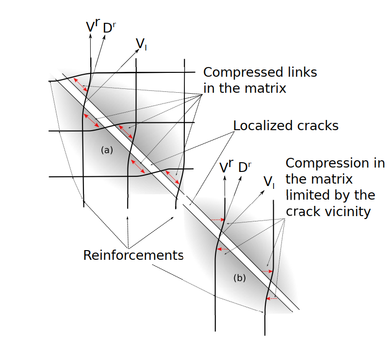
Figure 1: a) Mechanisms ensuring the Dowel effect, b) Cases of a more limited effect [Sellier, 2018]
It should be noted that this effect is allowed by the confinement zones developed between the reinforcements and the concrete as on the -a. If the number of frames is more limited (-b), the impact of this Dowel effect is greatly reduced [Sellier, 2018].
Finally, it should be noted that in the case of large elements, the representation of cracking is often not explicit. However, it is possible for these reinforced elements, and by considering the length of anchoring the steel and the maximum distance between two cracks, to obtain the number of localized cracks.
2.2. Behavioral law of the axial contribution of the frame#
The contribution of the frame is considered in its axial direction only. The behavioral law that defines it allows the consideration of plasticity and relaxation. The deformation of the frame is broken down according to its plastic part \({\epsilon }^{r,\mathit{pl}}\), and its elastic and permanent relaxation part, \({\epsilon }^{r,K}\) and \({\epsilon }^{r,M}\).
In addition, it is also possible to consider active reinforcement densities by considering an initial prestress value \({\sigma }_{0}^{r}\) such as:
The plastic deformation is evaluated by a criterion function making it possible to take into account the work hardening of the reinforcement. Considering the work-hardening modulus and the elastic limit, respectively \({H}^{r}\) and \({f}_{y}^{r}\), the criterion function is written as:
:math:`{f}^{r}= |
{sigma }^{r}-{H}^{r}{epsilon }^{r,mathit{pl}} |
-{f}_{y}^{r}le 0` |
2.2.1. Relaxation#
As seen in equation (), the model makes it possible to consider prestress. Since the present model has structural calculation purposes, relaxation phenomena must therefore be considered. These being strongly impacted by the initial voltage value as well as by the temperature [Ajimi et al., 2017], a relaxation model considering these impacts was implemented by [Chhun et al., 2018] [Chhun, 2017]. In the same way as the creep model implemented for concrete [CF notice aster RGI_BETON], this one is ensured by various coefficients impacting the instantaneous characteristics of the reinforcements in question. The model is composed of a first elastic part providing the instantaneous behavior, followed by a Kelvin stage ensuring the portion of visco-elastic deformations, and a third level directing the portion of permanent deformation, provided by a Maxwell module ().
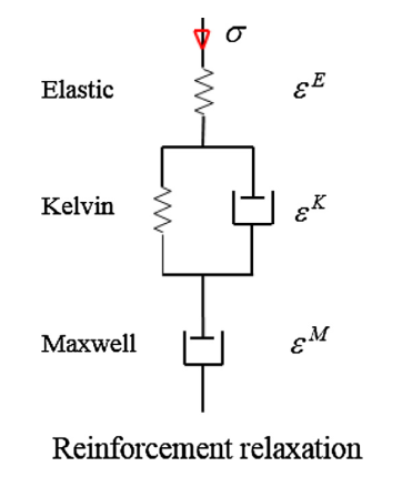
Figure 2: Idealized rheological diagram of the relaxation model from [Chhun, 2017]
2.2.1.1. Maxwell’s floor#
The permanent part of the relaxation is evaluated in a manner similar to that used by/in [:ref:` [Sellier et al., 2016 < [Sellier et al., 2016>`]/[Code_Aster [R7.01.36]]] for modeling permanent creep deformations. It is evaluated according to the elastic deformation ratio \({\epsilon }^{r,\mathit{el}}\) divided by the product of Maxwell’s characteristic time \({\tau }^{r,M}\), material parameter, and by the consolidation coefficient \(\mathit{Cc}\):
With \(\mathit{Cc}\) as a function of the viscous deformation reached at the current step, and of a coefficient k, relaxation amplitude coefficient:
In this equation, k makes it possible to consider the non-linear impact of temperature (T) and load rate (M) on the relaxation phenomenon:
With:
\({k}_{\mathit{ref}}\), parameter representing the relaxation capacity of the material, obtained by considering the parameters \({\epsilon }_{\mathit{ref}}^{K}\) and \({\sigma }_{\mathit{ref}}\), respectively the relaxation reference potential and the charge rate at which this potential has been fixed, such as:
\({k}^{M}\), allowing to consider the non-linear amplification of the relaxation rate with the load rate:
\(\mu\) being the load rate defined according to the elastic limit \({f}_{y}\) such that:
:math:`mu =frac{ |
sigma |
}{{f}_{y}}` |
and \({\mu }^{\mathit{cr}}\) the critical load rate, reflecting the non-linear tendency of the material to increase its relaxation rate with the increase in the load rate, a function of \(\chi\) nonlinear relaxation coefficient (defined such that the trend is linear for \(\chi =1\) and becoming non-linear for and becoming non-linear for \(\chi >1\), cf)
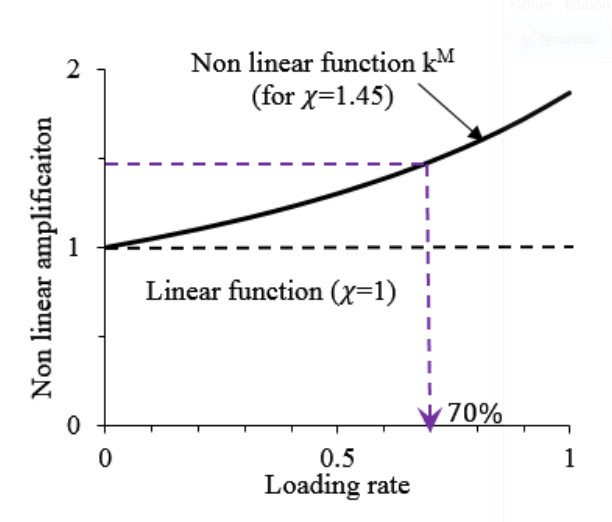
Figure 3: Nonlinear amplification function \({k}^{M}\) from [Chhun, 2017]
\({k}^{T}\), coefficient directing the acceleration of relaxation with increasing temperature, and ensuring non-linear evolution for a large load level:
With \({A}_{\mathit{ref}}^{T}\) reference value for the thermal activation coefficient, \(\gamma\) coupling coefficient for the impact of stresses on activation energy, \({\mu }^{\mathit{TM}}\) the charge rate that can modify thermal activation. Considering \({\mu }^{\mathit{thr}}\) the minimum charge rate threshold to impact the thermal activation coefficient fixed at 0.7, \({\mu }^{\mathit{TM}}\) is written as:
: label: eq-21
{mu} ^ {mathit {TM}}} (t+mathit {dt}) =mathit {dt}) =mathit {max} ({mu} ^ {mathit {TM}} (t),mu (t+mathit {dt}), {mathit {dt}})
2.2.1.2. Kelvin Floor#
Regarding viscoelastic behavior, and as developed by [Chhun et al., 2018], this one is ensured by a Kelvin module (). In the same way as permanent deformations, they are also affected by temperature:
With \({\tau }^{r,k}\) and \({\mathrm{\Psi }}^{k}\) respectively the characteristic time for the Kelvin deformations and the rate of this relaxation with respect to the elastic deformation, a function of reference values and of the \({k}^{T}\) thermal activation multiplier coefficient defines in equation ():
It should be noted that this part of the model was validated at the scale of the laboratory structure and applied on a large-scale structure [Chhun, 2017].
2.2.2. Adhesion: steel, concrete#
In the version of this model, the hypothesis of perfect adhesion is made between the two materials steel and concrete. In this way, the total axial deformation of the reinforcement is evaluated from its assumed elongation, determined from the concrete deformation matrix \(\overline{\overline{\epsilon }}\) such that:
With \({\epsilon }_{r}\) the axial deformation of the frame:
And \({\gamma }_{r}\) shear deformation
: label: eq-27
{gamma} _ {r} =Vertoverline {overline {epsilon}}vec {{V} ^ {r}} - {epsilon} _ {r}vec {{V}}vec {{V} ^ {r}}Green
It should be noted that taking into account a shift in this interface is possible but not implemented in this present model. This requires non-local calculations and is not shown here but can be found in [Sellier, and Millard, 2019].
2.3. Summary of the material parameters of RGI_BETON_BA#
In addition to the parameters of RGI_BETON, it is necessary to provide the following parameters (the gray parameters must be adjusted for each new material):
Parameter |
Significance |
Symbol |
Usual value |
Unit |
|
YOUM |
Young’s modulus specific to concrete |
\({E}^{\mathit{be}}\) |
15-40 |
|
|
NUM |
Poisson’s ratio specific to concrete |
\({\nu }^{\mathit{be}}\) |
0.2 |
||
NREN |
Total number of density considered |
\({N}^{r}\) |
[0 ; 5] |
||
ROA (i) |
Surface density |
\({\rho }^{r}\) |
0.01 |
m²/m² |
|
DEQ (i) |
Equivalent diameter |
\({\mathit{Deq}}^{r}\) |
|
m |
|
VR (i) 1 |
Projection of the frame direction according to \(\vec{x}\) |
|
1.0 |
||
VR (i) 2 |
Projection of the direction of the frame according to \(\vec{y}\) |
|
|||
VR (i) 3 |
Projection of the frame direction according to \(\vec{z}\) |
|
|||
YOR (i) |
Young’s Modulus |
\({E}^{r}\) |
200,000 |
|
|
SYR (i) |
Elastic limit |
\({f}_{y}^{r}\) |
|
MPa |
|
HPL (i) |
Work hardening module |
\({H}^{r}\) |
|
MPa |
|
TYR (i) |
Interface constraint |
\({\tau }^{r\mathrm{,1}}\) |
6 |
|
|
TMR (i) |
Irreversible characteristic times for creep (Maxwell) |
\({\tau }^{r,M}\) |
0.1 |
Days |
|
TKR (i) |
Reversible characteristic times for creep (Kelvin) |
\({\tau }^{r,K}\) |
0.1 |
Days |
|
PRE (i) |
Initial prestress (imposed as initial stress at the first step) |
\({\sigma }_{0}^{r}\) |
|
||
EKR (i) |
Characteristic deformation for relaxation |
\({\epsilon }_{\mathit{ref}}^{K}\) |
1e-4 |
||
SKR (i) |
Characteristic constraint for setting |
\({\sigma }_{\mathit{ref}}\) |
1260 |
|
|
XFL (i) |
Exhibitor for thermal activation of relaxation |
\({n}^{r}\) |
2, 55 |
||
XNR (i) |
Nonlinear relaxation coefficient |
\(\chi\) |
1.216 |
||
TTR (i) |
Reference temperature for setting \({\tau }^{r,M}\) |
|
38 |
°C |
|
CTM (i) |
Coupling coefficient for the impact of constraints on activation energy |
\(\gamma\) |
4, 8 |
||
ATR (i) |
Reference value for thermal activation coefficient |
\({A}_{\mathit{ref}}^{T}\) |
1, 5e-4 |
||
MUS (i) |
Threshold beyond which thermal activation becomes a function of the charge rate |
\({\mu }^{\mathit{thr}}\) |
0, 7 |
||
YKY (i) |
Reversible relaxation reduction coefficient evaluated at \({T}^{\mathit{ref}}\) |
\({\mathrm{\Psi }}_{\mathit{ref}}^{k}\) |
100 |