1. Theoretical formulation#
1.1. 1D vision of the behavior of the Iwan model#
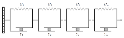
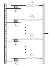
A purely 1D description of the Iwan model consists of a parallel or serial arrangement of Jenkin elements, each element being composed of a spring and a perfectly plastic friction pad (Coulomb criterion) in series (Figure 1). The arrangement of the elements and the parameters of the model determine the shape of the cyclic shear response.
|
|
Series-parallel model |
Parallel-serial model |
Figure 1.1-1: Iwan 1D rheological models [] |
|
1.2. 3D formulation of the Iwan model#
During the 3D description of the behavior, each element is associated with a load surface, defined from the deviatoric stress associated with each mechanism. We therefore go from a 1D description of the shear behavior to a 3D description of the deviatoric behavior based on the stress and deformation invariants, defined in the following way:
Constraint deviator: \(\text{q}={\mathrm{S}}_{\text{V}\text{M}}^{\text{3}\text{D}}=\sqrt{\frac{\text{3}}{\text{2}}\text{S}\mathrm{:}\text{S}}\) |
: label: eq-4
textrm {Volume deformation:} {mathrm {epsilon}} _ {v} =mathit {tr}left (mathrm {epsilon}right)
Deviatoric deformation: \({\text{q}}_{\text{n}}={\left(\text{S}-{\text{X}}_{\text{n}}\right)}_{\text{V}\text{M}}^{\text{3}\text{D}}=\sqrt{\frac{\text{3}}{\text{2}}(\text{S}-{\text{X}}_{\text{n}})\mathrm{:}(\text{S}-{\text{X}}_{\text{n}})}\) |
For a series-parallel arrangement, when the stress applied exceeds the limiting stress \({Y}_{n}\) of the \(n\) mechanism, there is work hardening of this mechanism and the associated stress remains equal to the limit stress, i.e. only kinematic work hardening is associated with each mechanism of the model. The model allows great flexibility in describing behavior, in particular through the possibility of direct use of test data in the laboratory. The error associated with describing cyclic behavior depends directly on the number of load surfaces and their arrangement. However, the greater the number of mechanisms, the more numerically expensive the system to be solved is, despite the transition from a tensor system to a scalar system (section 2).
The model is based on the theory of multi-mechanism elastoplasticity. In a series-parallel description, it assumes an additive and independent decomposition of the deformations on the work hardening mechanisms:
For each mechanism, the model considers an additive decomposition of the total deformation tensor \(\text{ε}\) into an elastic part \({\text{ε}}_{\text{n}}^{\text{e}}\) and a plastic part \({\mathrm{\epsilon }}_{n}^{p}\):
The stress-strain relationship is written directly from the 4th order elasticity tensor, \(C\) *.* The elasticity is therefore linear and the model does not allow the effect of confinement to be taken into account in the elastic constants.
Since the model only describes deviatoric behavior, the volume response is assumed to be linear elastic:
where \(>\) is the compression module.
In the following, the various ingredients necessary to describe the law of behavior in an elasto-plastic framework are described, namely:
Load surface \(\text{f}\): defines the area in the stress space within which the behavior is linear elastic (\(\text{f}<0\) or \(\text{f}=0\) and \(d\text{f}<0\)) and where the behavior is plastic (\(\text{f}=0\) and \(d\text{f}>0\)).
Flow law: rule defining the plastic deformation increment, in a generic way \({\dot{\mathrm{\epsilon }}}^{p}=\dot{\mathrm{\lambda }}\mathrm{\Psi }\), where \(\dot{\mathrm{\lambda }}\) is the plastic multiplier and \(\mathrm{\Psi }\) the flow law.
1.2.1. Charging surface description#
The load area of each mechanism is written as follows:
With \({Y}_{n}\) a limit constant from which the \(>\) mechanism works. This value is chosen from a pure shear test, by associating each \(>\) work hardening mechanism with a pair of values \(\left({\mathrm{\gamma }}_{n},{\mathrm{\tau }}_{n}\right)\) with \(\mathrm{\gamma }=2{\mathrm{\epsilon }}_{\mathit{ij}}\), \(\text{i}\ne \text{j}\). So \({Y}_{n}\) is directly obtained from \({\mathrm{\tau }}_{n}\) by the following relationship:
The value of \({q}_{n}\) is the deviatoric constraint associated with the \(n\) mechanism, defined as follows:
\({\text{q}}_{\text{n}}={\left(\text{S}-{\text{X}}_{\text{n}}\right)}_{\text{V}\text{M}}^{\text{3}\text{D}}=\sqrt{\frac{\text{3}}{\text{2}}(\text{S}-{\text{X}}_{\text{n}})\mathrm{:}(\text{S}-{\text{X}}_{\text{n}})}\) |
The tensor \({\text{X}}_{\text{n}}\) represents the kinematic work hardening of the \(\text{n}\) mechanism. It is obtained from the expression defined by Prager:
With \({C}_{n}\) a model parameter determined from a monotonic shear test. Because \({C}_{n}\) is constant, we consider work hardening to be linear.
1.2.2. Description of the flow law#
The plastic deformation increments for each \(n\) mechanism are obtained from the plastic multiplier \({\dot{\mathrm{\lambda }}}_{n}\) and the flow law \({\mathrm{\Psi }}_{n}\):
Since the model assumes an associated flow, the flow law is obtained directly from the load surface:
The plastic multiplier associated with each mechanism is obtained from the consistency equation, i.e. \({\dot{f}}_{n}=0\):
With:
The calculation of the plastic multiplier is explained in section 2.
1.2.3. Calculation of work hardening parameters \({C}_{n}\)#
The determination of the kinematic work hardening parameters \({C}_{n}\) is made from a pure shear stress path (\(\mathrm{\Delta }p=0\)). Assume the known answer for this stress path from an initial state with zero deviatoric stress and zero plastic deformation. In this case:
From \(>\) \(\left({\mathrm{\gamma }}_{n},{\mathrm{\tau }}_{n}\right)\) couples, we can estimate the value of \({C}_{n}\) recursively with the following expression:
The calculation of the kinematic work hardening parameters \({C}_{n}\) is done in the @InitLocalVars block of Mfront.