3. Parameters of the law#
The damagable reinforced concrete slab model GLRC_DM therefore needs parameters characteristic of elasticity, supplemented by 6 parameters to describe the damage behavior: \({k}_{0}\), to define the elastic limit, \(\alpha\) to determine the participation of flexure (see § 2.2), \({\gamma }_{\mathrm{mt}}\), \({\gamma }_{\mathrm{mc}}\) and \({\mathrm{\alpha }}_{c}\), \({\gamma }_{f}\) to describe the nonlinear response. All of these parameters can be identified from monotonous uniaxial pure tensile and flexural tests. Some of them are replaced in the Code_Aster dataset by more « meaningful » parameters, see § 3.2.5 below.
It is possible to proceed either from simple analytical estimates (which give orders of magnitude) or from a realignment on a response curve provided by another behavior model, possibly by integrating compromises.
The approach is described in the paragraphs below and an overview is given in § 3.2.5.
3.1. Identification of linear elastic behavior parameters#
In this model, it is assumed that the reinforced concrete medium is homogenized and it is left to the user to choose (calculate or measure) the parameters: \({E}_{\mathrm{eq}}^{m}\) (effective Young’s modulus in membrane), \({E}_{\mathrm{eq}}^{f}\) (effective Young’s modulus in flexure), \({\nu }_{m}\) (effective Young’s modulus in flexure), (effective Poisson’s ratio in membrane), and \({\nu }_{f}\) (effective Poisson’s ratio in flexure). The following relationships are applied to determine the Lamé coefficients \({\lambda }_{m}\), \({\mu }_{m}\) and \({\lambda }_{f}\), \({\mu }_{f}\):
The relationships above are not interchangeable by F ↔ M for the membrane and flexure parameters, since in membrane the relationships correspond to the general case (3D elasticity) and the condition of plane stresses is treated within the formulation of the model, while for flexure we immediately adopted 2D elasticity with plane stresses. In the elastic domain we thus have:
\(\begin{array}{}{N}_{\alpha \beta }=\frac{{E}_{\mathrm{eq}}^{m}h}{1-{\nu }_{m}^{2}}({\nu }_{m}\mathrm{.}\mathrm{tr}\epsilon \mathrm{.}{\delta }_{\alpha \beta }+(1-{\nu }_{m}){\epsilon }_{\alpha \beta })\\ {M}_{\alpha \beta }=\frac{{E}_{\mathrm{eq}}^{f}{h}^{3}}{12(1-{\nu }_{f}^{2})}({\nu }_{f}\mathrm{.}\mathrm{tr}\kappa \mathrm{.}{\delta }_{\alpha \beta }+(1-{\nu }_{f}){\kappa }_{\alpha \beta })\end{array}\)
\(\alpha\) and \(\beta\) being indices ranging from 1 to 2.
By default \({E}_{\mathrm{eq}}^{m}={E}_{\mathrm{eq}}^{f}=E\) and \({\nu }_{m}={\nu }_{f}=\nu\), where \(E\) and \(\nu\) are the elastic coefficients entered in the command file under the keyword ELAS. On the other hand, as reinforced concrete is not a homogeneous material, the effective value of \({E}_{\mathrm{eq}}^{f}\) may be different from \({E}_{\mathrm{eq}}^{m}\). Therefore, the user is given the possibility of entering values \({E}_{\mathrm{eq}}^{f}\) and \({\nu }_{f}\) (EF and (EF and NUF under the keyword factor GLRC_DM) different from \(E\) and \(\nu\), which in this case are only used to describe membrane elasticity.
The plane stress condition for membrane \({\sigma }_{\mathrm{zz}}=0\) is satisfied as described in § 2.3.
Note:
In [eq. ], we get a different relationship between \({\lambda }_{f}\) , \({\nu }_{f}\) , and \({E}_{\mathrm{eq}}^{f}\) on the one hand, and between \({\lambda }_{m}\) , \({\nu }_{m}\) and \({E}_{\mathrm{eq}}^{m}\) on the other hand. This difference is directly linked to the different consideration of the plane stress condition in membrane and in flexibility. More particularly, we define \({E}_{\mathrm{eq}}^{f}\) and \({\nu }_{f}\) through a pure flexure test, where \({\kappa }_{\mathrm{yy}}=-{\nu }_{f}{\kappa }_{\mathrm{xx}}\), and \({M}_{\mathrm{ij}}=0\) , except \({M}_{\mathrm{xx}}\ne 0\). We then use the following equations to find the relationship between \({\lambda }_{f}\) , \({\mu }_{f}\) and \({E}_{\mathrm{eq}}^{f}\) , \({\nu }_{f}\) :
\({M}_{\mathrm{yy}}=({\lambda }_{f}(1-{\nu }_{f})-2{\mu }_{f}{\nu }_{f}){\kappa }_{\mathrm{xx}}=0\)
and
\({M}_{\mathrm{xx}}=({\lambda }_{f}(1-{\nu }_{f})-2{\mu }_{f}){\kappa }_{\mathrm{xx}}=\frac{{E}_{\mathrm{eq}}^{f}{h}^{3}}{12}{\kappa }_{\mathrm{xx}}\)
from where we get:
\({E}_{\mathrm{eq}}^{f}=\frac{12}{{h}^{3}}({\lambda }_{f}(1-{\nu }_{f})+2{\mu }_{f})\) and \({\lambda }_{f}(1-{\nu }_{f})-2{\mu }_{f}{\nu }_{f}=0\) ( 3.1-2 )
By solving [eq.], we have the relationships expressed in [eq. ] .
The identification of the elastic parameters \({E}_{\mathrm{eq}}^{m}\), \({\nu }_{m}\), \({E}_{\mathrm{eq}}^{f}\) and \({\nu }_{f}\) of the model from the characteristics of concrete and steels is based on two load cases: pure traction and pure bending.
Let us consider the following characteristics for concrete: Young’s modulus \({E}_{b}\), Poisson’s ratio, Poisson’s ratio \({\nu }_{b}\),, Poisson’s ratio, and for steels: Young’s modulus \({E}_{a}\), Poisson’s ratio \({\nu }_{a}\), total cross section per linear meter (for the two sheets, assumed to be symmetric in thickness and identical in both directions) \({S}_{a}\), position \(h\) relative of a sheet in thickness \({\chi }_{a}\in \left]\mathrm{0,}1\right[\).
Thus, using the uniaxial test using pure elastic tension, we obtain:
From where (keywords E and NU):
It is observed that this identification produces an error in the flat elastic shear stiffness of the slab, a case for which steels do not contribute (these are welded rod grids), which makes the homogenized behavior orthotropic and not isotropic. In fact, with the values [eq. ]:
If we prefer to provide priority identification on the case of plane elastic shear of the slab, and on the case of the response according to the pure direction of traction (therefore by accepting the error on the orthogonal Poisson effect), we obtain:
Care should be taken to ensure that this crude identification (not admissible thermodynamically compared to the pure tensile test) does not give fanciful values of \({\nu }_{m}\).
Then, using the uniaxial test in pure elastic flexuration, we obtain:
From where (EF keywords and NUF):
It is also observed that this identification produces an error on the stiffness in anticlastic elastic flexure \({M}_{\mathrm{xy}}\) of the slab (coefficient \({G}_{\mathrm{eq}}^{f}=\frac{{E}_{\mathrm{eq}}^{f}{h}^{3}}{24(1+{\nu }_{f})}\) instead of \({G}_{b}^{f}=\frac{{E}_{b}{h}^{3}}{24(1+{\nu }_{b})}\)), a case for which steels do not contribute.
3.2. Identification of parameters of damageable elastic behavior#
Since the way in which the parameters of linear elasticity are obtained is presented in § 3.1, it is proposed to calculate the damage parameters of the model from three tests: a pure tension test, a pure compression test and a pure uniaxial monotonic flexure test.
In this way, the values of the threshold \({k}_{0}\), of the three parameters relating to membrane effects (\({\gamma }_{\mathrm{mt}}\), \({\alpha }_{c}\) and \({\mathrm{\gamma }}_{\mathit{mc}}\)) are obtained independently of the two parameters relating to the effects of flexure (\(\alpha\), \({\gamma }_{f}\)).
3.2.1. Traction parameters (keywords NYT, GAMMA_T)#
3.2.1.1. Threshold for onset of damage during traction NYT#
In particular, for the pure uniaxial elastic traction at the onset of damage we can write the threshold value, cf. [eq.]:
\({f}_{{d}_{j}}={Y}_{j}^{m}-{k}_{0}={\epsilon }_{D}^{2}(\frac{{\lambda }_{m}}{4}{(1-2{\nu }_{m})}^{2}(1-{\gamma }_{\mathrm{mt}})+\frac{{\mu }_{m}}{2}(1-{\gamma }_{\mathrm{mt}}+{\nu }_{m}^{2}\frac{1-{\gamma }_{\mathrm{mc}}}{{\alpha }_{c}}))-{k}_{0}=0\)
\({\epsilon }_{D}\) being the elastic deformation at the onset of damage, then having \({\epsilon }_{\mathrm{yy}}=-{\nu }_{m}{\epsilon }_{D}={\varepsilon }_{\mathrm{zz}}\) and \({\xi }_{m}(x\mathrm{,0},0)=1\), hence:
having
\({N}_{D}=({\lambda }_{m}(1-2{\nu }_{m})+2{\mu }_{m}){\epsilon }_{D}={E}_{\mathrm{eq}}^{m}h{\epsilon }_{D}\)
Note:
We recall that \({\gamma }_{\mathrm{mt}}\le 1\) (cf. eq. ) and \({\gamma }_{\mathrm{mc}}\le 1\) so that the damage actually results in a weakening of the stiffness. We also observe on [eq. ] that we cannot have both \({\gamma }_{\mathrm{mt}}=1\) and \({\gamma }_{\mathrm{mc}}=1\) , because \({k}_{0}=0\) (the model has no elastic domain), or else we would have to give \({N}_{D}=\infty\) (keyword NYT) .
Continuing the analysis done in 3.1, just when damage occurred, the longitudinal stress in concrete is equal to:
\({E}_{b}{\epsilon }_{D}\frac{1-{\nu }_{b}{\nu }_{m}}{1-{\nu }_{b}^{2}}\)
so that we can express the threshold \({N}_{D}\) (keyword NYT) with the concrete crack limit \({\sigma }_{b}^{t}\) under tension, assuming the local criterion \({\sigma }_{\mathrm{xx}}\le {\sigma }_{b}^{t}\) is valid:
3.2.1.2. Tensile stiffness degradation parameter GAMMA_T#
Parameter \({\gamma }_{\mathit{mt}}\) is equal to the ratio between the slope corresponding to the stiffness of the damaged phase, provided by the keyword PENTE/TRACTIONdans DEFI_GLRC and the slope corresponding to the elastic stiffness.
As a reminder (see U4.42.06), three methods called RIGI_ACIER, PLAS_ACIER and UTIL are available. These three slope calculations make it possible to set up three different calibration methods according to the material properties entered for traction. In the case where the elastic limit of steels is not known, the adjustment methods RIGI_ACIER, i.e. post-elastic slope equal to the steels” stiffness recovery slope, and UTIL, i.e. post-elastic slope cuts the steels stiffness recovery slope at a maximum deformation whose value is imposed by the user, are accessible (this method is not suitable for maximum deformations smaller than the trough of the curve). for reference, see). In the case where the limit of elasticity of steels is known, it is possible to use the method of adjusting to the limit of plasticity of steels (PLAS_ACIER). The various recalibration methods are illustrated by the following figures.

Figure 3.2.1.2-a : Traction curve ( GLRC_DM vs Reference) Recalibration PENTE = RIGI_ACIER

Figure 3.2.1.2-b: Traction Curve (GLRC_DM vs Reference) Adjustment PENTE = UTIL

Figure 3.2.1.2-c : Traction curve ( GLRC_DM vs Reference) Recalibration PENTE = PLAS_ACIER
3.2.1.3. Pure uniaxial distortion case#
Let’s check the effect of these parameters on the occurrence of damage following a loading of pure distortion elastic \({\epsilon }_{\mathrm{xy}}=\tilde{{\epsilon }_{1}}=-\tilde{{\epsilon }_{2}}\), with \({\epsilon }_{\mathrm{xx}}={\epsilon }_{\mathrm{yy}}=0\). So: \({N}_{\mathrm{xy}}=\tilde{{N}_{1}}=-\tilde{{N}_{2}}=2{\mu }_{m}{\epsilon }_{\mathrm{xy}}\). The damage onset threshold [eq.] with model GLRC_DM is reached for the shear force:
\({N}_{\mathrm{xy}}^{D}=2\frac{\sqrt{2{\mu }_{m}{k}_{0}}}{\sqrt{1+{\alpha }_{c}-{\gamma }_{\mathrm{mc}}-{\gamma }_{\mathrm{mt}}{\alpha }_{c}}}=\frac{{N}_{D}}{1+{\nu }_{m}}\cdot \sqrt{\frac{(1-{\nu }_{m})(1+2{\nu }_{m})(1-{\gamma }_{\mathrm{mt}})+{\nu }_{m}^{2}(1-{\gamma }_{\mathrm{mc}})/{\alpha }_{c}}{1+{\alpha }_{c}-{\gamma }_{\mathrm{mc}}-{\gamma }_{\mathrm{mt}}{\alpha }_{c}}}\)
It may be useful to compare this prediction with the one obtained with the concrete model ENDO_ISOT_BETON [R7.01.04], [2.3.2.3], with the concrete crack limit \({\sigma }_{b}^{t}\) under tension:
\({{N}_{\mathrm{xy}}^{D}}_{\mathrm{EIB}}=2{\sigma }_{b}^{t}h\sqrt{\frac{(1-{\nu }_{b})(1+2{\nu }_{b})}{{(1+{\nu }_{b})}^{2}}}=2{N}_{D}\frac{{E}_{b}(1-{\nu }_{b}{\nu }_{m})}{{E}_{\mathrm{éq}}^{m}(1-{\nu }_{b}^{2})}\cdot \sqrt{\frac{(1-{\nu }_{b})(1+2{\nu }_{b})}{{(1+{\nu }_{b})}^{2}}}\)
Note:
In any combined situation (compression+shear, etc.) in a pure membrane, the expression of the first damage threshold \({Y}_{j}^{m}={k}_{0}\) of the model GLRC_DM, cf. [eq. ], as a function of membrane efforts \({N}_{\mathrm{xx}},{N}_{\mathrm{xy}}\mathrm{...}\) , consists of the same monomials as the « usual » criterion in plane stresses of the concrete material considered not to withstand beyond \({\sigma }_{b}^{t}\). This comes from the choice of the formulation of the model GLRC_DMen membrane, in direct connection with the model ENDO_ISOT_BETON.
3.2.2. Compression settings (keywords NYC, GAMMA_C, ALPHA_C)#
In compression, three parameters are to be determined: \({N}_{C}\), \({\alpha }_{c}\) and \({\gamma }_{\mathrm{mc}}\). Three equations are used to do this.
The first comes from the formulation of the model. If a pure uniaxial compression test is considered, the value of the first damage threshold, cf. [eq.], is written by designating \({N}_{C}\) the corresponding normal force:
\({k}_{0}=\frac{{N}_{C}^{2}}{4{E}_{\mathrm{éq}}^{m}h(1+{\nu }_{m})}\cdot ((1-{\nu }_{m})(1+2{\nu }_{m})\frac{1-{\gamma }_{\mathrm{mc}}}{{\alpha }_{c}}+{\nu }_{m}^{2}(1-{\gamma }_{\mathrm{mt}}))\)
We must therefore necessarily have the relationship:
\(\frac{{N}_{C}^{2}}{{N}_{D}^{2}}=\frac{{\alpha }_{c}(1-{\nu }_{m})(1+2{\nu }_{m})(1-{\gamma }_{\mathrm{mt}})+{\nu }_{m}^{2}(1-{\gamma }_{\mathrm{mc}})}{(1-{\nu }_{m})(1+2{\nu }_{m})(1-{\gamma }_{\mathrm{mc}})+{\alpha }_{c}{\nu }_{m}^{2}(1-{\gamma }_{\mathrm{mt}})}\)
So, we get the expression for \({\alpha }_{c}\) in terms of \({\gamma }_{\mathrm{mc}}\), \({\gamma }_{\mathrm{mt}}\), and \({N}_{D}\), \({N}_{C}\):
Note:
It is required \({\gamma }_{\mathrm{mc}}\le 1\) , just as \({\gamma }_{\mathrm{mt}}\le 1\), cf. [eq.]. We also recall, cf. [eq. ], that one cannot have both \({\gamma }_{\mathrm{mt}}=1\) and \({\gamma }_{\mathrm{mc}}=1\) at the same time. From [eq. ], we obtain the necessary condition, regardless of \({\alpha }_{c}\) :
\(\mid {N}_{C}\mid \le {N}_{D}\frac{\sqrt{(1-{\nu }_{m})(1+2{\nu }_{m})}}{{\nu }_{m}}\)
Equality in the relationship above leads to \({\gamma }_{\mathrm{mc}}=1\) .
For reinforced concrete, has \({\nu }_{m}\approx \mathrm{0,2}\) , this condition is written as: \(\mid {N}_{C}\mid <\mathrm{5,2}{N}_{D}\) .
The second equation comes from an additional condition that we impose: we aim for the same maximum damage in tension and in compression. 418 corresponds to the greatest loss of stiffness, both in tension (denoted by. ») and in compression (denoted by.
Finally, a variable \({N}_{\mathit{CU}}\) is introduced which corresponds to the ultimate resistance of the compression section, based on the height h of the shell, and from the value of the average compression resistance \({F}_{\mathit{CJ}}\) and \({ϵ}_{\mathit{C1}}\) the corresponding deformation.
\({N}_{\mathit{CU}}=h{F}_{\mathit{CJ}}+{E}_{a}{S}_{a}\cdot {ϵ}_{\mathit{C1}}\)
The compression threshold \({N}_{C}\) is then linked to the ultimate compression limit \({N}_{\mathit{CU}}\) via the equation:
The aim is to achieve the same maximum damage in tension and in compression. \({d}_{\mathit{max}}\) must therefore make it possible to achieve the greatest loss of stiffness, both in traction (noted \({\xi }_{{t}_{\mathit{min}}}\)) and in compression (noted \({\xi }_{{c}_{\mathit{min}}}\)). In compression, the maximum damage makes it possible to reach compression peak \({N}_{\mathit{CU}}\). In traction, it makes it possible to reach the point of plasticization of steels.
Solving the equation [eq. ] gives the maximum damage value \({d}_{\mathit{max}}\) .
\({d}_{\mathit{max}}=\frac{{S}_{a}{\sigma }_{\mathit{ya}}-{N}_{D}}{{N}_{D}\ast {\gamma }_{\mathit{mt}}}\)
In the case where the value obtained for \({d}_{\mathit{max}}\) is positive, we get:
\({\alpha }_{c}=\frac{{d}_{\mathit{max}}{N}_{C}(1-{\gamma }_{\mathit{mc}})}{h{E}_{m}{ϵ}_{\mathit{C1}}-{N}_{\mathit{CU}}}\) If you have to have \({N}_{\mathit{CU}}<h{E}_{m}{ϵ}_{\mathit{C1}}\)
and
\(\frac{{d}_{\mathit{max}}{N}_{C}}{h{E}_{m}{ϵ}_{\mathit{C1}}-{N}_{\mathit{CU}}}=\frac{({N}_{D}^{2}{\nu }_{m}^{2}-{N}_{C}^{2}(1-{\nu }_{m})(1+2{\nu }_{m}))}{(1-{\gamma }_{\mathit{mt}})({N}_{C}^{2}{\nu }_{m}^{2}-{N}_{D}^{2}(1-{\nu }_{m})(1+2{\nu }_{m}))}\)
This last equation is a cubic equation \({N}_{C}\)
In the case where \({d}_{\mathit{max}}<0\), we modify the calculation of \({\gamma }_{\mathit{mt}}\), by imposing
\({\gamma }_{\mathit{mt}}=0\)
and the equation [eq. ] is modified by
\({ϵ}_{\mathit{tmax}}=\frac{{\sigma }_{\mathit{ya}}}{{E}_{a}}\) \(\frac{1}{1+{d}_{\mathit{max}}}=\frac{{S}_{a}{\sigma }_{\mathit{ya}}}{{\mathit{hE}}_{m}{ϵ}_{\mathit{tmax}}}\)
with
so we have \({d}_{\mathit{max}}=\frac{{\mathit{hE}}_{m}}{{S}_{a}{\sigma }_{\mathit{ya}}}-1\).
3.2.3. Flexion parameters (keywords MYF, GAMMA_F)#
3.2.3.1. Options RIGI_ACIER and PLAS_ACIER#
In pure uniaxial elastic flexion only one damage mechanism is activated, depending on its meaning, positive or negative. Here we choose positive inflection, for which we always have \({f}_{{d}_{1}}>{f}_{{d}_{2}}\). The maximum elastic curvature value \({\kappa }_{\mathrm{xx}}\) at the onset of damage is noted \({\kappa }_{D}\) (\({\kappa }_{\mathrm{yy}}=-{\nu }_{f}{\kappa }_{\mathrm{xx}}\)), such that only the threshold \({f}_{{d}_{1}}=0\) can be reached, while \({f}_{{d}_{2}}<0\) for each point of this loading trajectory, cf. [eq.]:
\({f}_{{d}_{1}}={Y}_{1}^{f}-{k}_{0}={\kappa }_{D}^{2}\frac{(1-{\gamma }_{f})}{\alpha }(\frac{{\lambda }_{f}}{2}{(1-{\nu }_{f})}^{2}+{\mu }_{f})-{k}_{0}\)
from where:
having
\({M}_{D}=({\lambda }_{f}(1-{\nu }_{f})+2{\mu }_{f})\mathrm{.}{\kappa }_{D}=\frac{{E}_{\mathrm{eq}}^{f}{h}^{3}}{12}{\kappa }_{D}\)
As the reinforced concrete plate is assumed to be symmetric with respect to the middle sheet, identification is only necessary for positive deflection (negative deflection giving the same value).
Continuing the analysis done in § 3.1, just when the damage occurs, the longitudinal stress in the concrete applies to the wall of the plate (we know that then the damage progresses immediately in a good part of the thickness of the section):
\({E}_{b}{\kappa }_{D}h\frac{1-{\nu }_{b}{\nu }_{f}}{2(1-{\nu }_{b}^{2})}\)
so that we can express threshold \({M}_{D}\) with the concrete crack limit \({\sigma }_{t}^{b}\):
This value is used for the RIGI_ACIER and PLAS_ACIER settings of the PENTE/FLEXION operand of DEFI_GLRC.
Parameter \({\mathrm{\gamma }}_{f}\) is equal to the ratio between the slope corresponding to the stiffness of the damaged phase, provided by the keyword PENTE/FLEXIONdans DEFI_GLRC, and the slope corresponding to the elastic stiffness. The options RIGI_ACIER and PLAS_ACIER correspond to the behavior presented for traction at the 3.2.1.2.
In order to more accurately represent the flexural behavior of reinforced concrete for a narrower range of curvature, two methods are introduced for the identification of flexural parameters.
These two methods are based on the prior identification of the theoretical curvature-bending curve of the section. This theoretical curve is determined from the theory of the plane section.
The response of the section is calculated by integrating the responses on the height of the section.
The response hypotheses for each material are as follows:
Nonlinear response of concrete defined by the tension limit SYT, the compression limit SYC and the parameter c which determines the value of the slope of the tensile behavior of concrete after cracking. We remember c=5, that is to say that the slope after cracking is equal to -0.2 \({p}_{\mathit{elas}}\), where \({p}_{\mathit{elas}}\) is the elastic slope. This is a compromise evaluated from numerical tensile tests with law ENDO_ISOT_BETON for classes of concrete commonly used by engineering. We add the hypothesis that the compression limit is greater than the tension limit (in absolute value) \(\mid \mathit{SYC}\mid >\mid \mathit{SYT}\mid\).
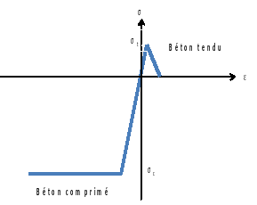
Figure 3.2.3.1-a :: **Behavior of concrete for calculating the curvature-moment curve
Elasto-plastic response of steel defined by the SY parameter
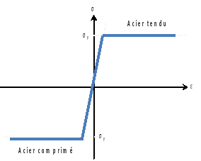
Figure 3.2.3.1-b **: ****Behavior of concrete for calculating the curvature-moment curve
To determine the curvature-bending response, we start from the hypothesis of a resultant of zero axial force. For the data of a curvature, the value of the deformation at the neutral axis is determined in order to obtain a zero axial force resultant. This determination is carried out by making assumptions about the possible states (concrete cracking, compression limit reached, plasticization of steels… etc.). It does not require digital integration with a precision criterion, which makes its use safer and less expensive.
The moment is then determined from the values of the deformation at the neutral axis and the curvature.
Note:
In the case of modeling the section of the proposed shell, the flexural modulus obtained is equal to:
\({E}_{\mathit{eq}}^{f}=\frac{3}{h}{E}_{a}{S}_{a}{\chi }_{a}^{2}+{E}_{b}\)
It therefore differs from the module that takes into account the Poisson’s ratio [eq. ] .
To ensure the consistency of the formulas and to obtain the same results in elastic flexure, a modified Young’s modulus of concrete is used in calculating the response of the section via integration into the height.
\(\stackrel{̃}{{E}_{b}}={E}_{b}\cdot \frac{{E}_{b}h+3{E}_{a}{S}_{a}{\chi }_{a}^{2}}{{E}_{b}h+3{E}_{a}{S}_{a}{\chi }_{a}^{2}(1-{\nu }_{b}^{2})}\)
Two options are available for determining the bilinear approximation of the Curve-Curve Curve Curve Curve Curve Curve.
3.2.3.2. Option RIGI_INIT#
For identification option RIGI_INIT, the threshold bending moment corresponding to the onset of damage is defined as follows:
Starting from the point of initiation of the first crack \({M}_{D}\), we look for the smallest moment on the elastic curve, for which the difference from the theoretical curve exceeds 5%. This moment is used for the value \(\mathit{MYF}\).
The damage slope in pure uniaxial bending is then defined as the slope from the tangent to the theoretical moment-curve curve and passing through the defined threshold point.
Parameter \({\gamma }_{f}\) is then defined as the ratio of the damaging and elastic slopes.
Note:
For sections with little reinforcement, a negative damaging slope can be obtained. \({\gamma }_{f}<0\). In this case an alarm message is displayed, a slope \({\gamma }_{f}={10}^{-3}\) is imposed and the threshold moment \(\mathit{MYF}\) is reduced to satisfy the tangent condition to the theoretical curve.
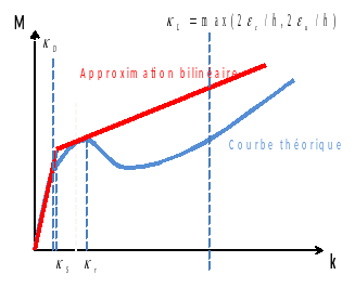
Figure 3.2.3.2-a : **Bilinear approximation in bending with the option** RIGI_INIT ****
To implement this option, the following steps are carried out:
For each curvature, in a curve interval \(\left[{\kappa }_{D},{\kappa }_{L}\right]\), the theoretical moment \(M\) and the tangent \(\mathit{dM}/d\kappa\) to the curve (\(d\kappa =({\kappa }_{L}-{\kappa }_{D})/1000\)) are determined. This tangent is obtained by finite difference.
Among the calculated values, we select the first curvature for which the deviation from the curve is greater than 5%.
To obtain the damage slope, we select the limit curvature \({\kappa }_{R}\) for which we minimize the difference between \(\mathit{dM}/d\kappa\) and the damage slope.
3.2.3.3. Option UTIL#
For identification option UTIL, the user defines a target curvature value using the KAPPA_FLEX keyword. The value of the curvature and the threshold moment \({\kappa }_{s}\) and \(\mathit{MYF}\) is then determined so as to minimize the area between the theoretical curve and the bilinear curve.
Note:
For sections with little reinforcement, a negative damage slope can be obtained. \({\gamma }_{f}<0\). In this case an alarm message is displayed, a slope \({\gamma }_{f}={10}^{-3}\) is imposed and the threshold moment \(\mathit{MYF}\) is defined at the concrete crack limit, i.e. \({M}_{D}\).
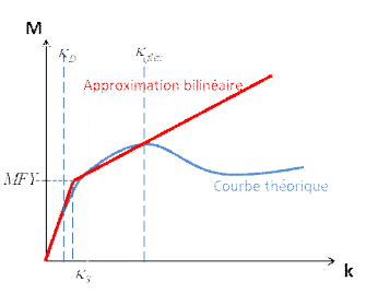
Figure 3.2.3.3-a : **Bilinear approximation in bending with the option** UTIL ****
To implement this option, the following steps are carried out:
For each curvature, in a curve interval \(\left[{\mathrm{\kappa }}_{D},{\mathrm{\kappa }}_{\mathit{flex}}\right]\) (1000 points), the theoretical moment \(M\) is determined and the area under the theoretical curve is calculated using the rectangle method, as well as the area under the bilinear curve.
The area under the curve is evaluated using bilinear approximations that guarantee the elastic slope calculated beforehand and that intersect the theoretical curve for \(\mathrm{\kappa }={\mathrm{\kappa }}_{\mathit{flex}}\): the threshold point is moved along the elastic slope and the damaged slope adjusted to pass through the theoretical curve.
We use the bilinear approximation which minimizes the difference between the area under its curve and that of the theoretical curve.
3.2.4. Uniaxial traction-flexure cases#
Let us verify the effect of these parameters on the occurrence of damage following a loading combining traction monotonic uniaxial and flexion concomitant uniaxial monotonic flexion. For each damage variable, the thresholds are written as:
\(\begin{array}{}{k}_{0}\ge {Y}_{1}=\\ {\epsilon }_{\mathrm{xx}}^{2}(\frac{{\lambda }_{m}}{4}{(1-2{\nu }_{m})}^{2}(1-{\gamma }_{\mathrm{mt}})+\frac{{\mu }_{m}}{2}(1-{\gamma }_{\mathrm{mt}}+{\nu }_{m}^{2}\frac{1-{\gamma }_{\mathrm{mc}}}{{\alpha }_{c}}))+{\kappa }_{\mathrm{xx}}^{2}{\nu }_{f}^{2}{\mu }_{f}\frac{(1-{\gamma }_{f})}{\alpha }\end{array}\)
\(\begin{array}{}{k}_{0}\ge {Y}_{2}=\\ {\epsilon }_{\mathrm{xx}}^{2}(\frac{{\lambda }_{m}}{4}{(1-2{\nu }_{m})}^{2}(1-{\gamma }_{\mathrm{mt}})+\frac{{\mu }_{m}}{2}(1-{\gamma }_{\mathrm{mt}}+{\nu }_{m}^{2}\frac{1-{\gamma }_{\mathrm{mc}}}{{\alpha }_{c}}))+{\kappa }_{\mathrm{xx}}^{2}\frac{(1-{\gamma }_{f})}{\alpha }(\frac{{\lambda }_{f}}{2}{(1-{\nu }_{f})}^{2}+{\mu }_{f})\end{array}\)
It is easy to verify that \({Y}_{1}<{Y}_{2}\): the first damage appears on the \({d}_{2}\) variable as expected. Let’s use the results [eq.] and [eq.], so threshold \({Y}_{2}={k}_{0}\) is written:
It thus defines the elastic domain predicted by the model GLRC_DM in the positive \(({N}_{\mathrm{xx}},{M}_{\mathrm{xx}})\) quadrant in an elliptical form.
Continuing the analysis done in § 3.1, just when damage occurs, the longitudinal stress in concrete is equal to:
\(\frac{{E}_{b}}{1-{\nu }_{b}^{2}}({\epsilon }_{\mathrm{xx}}(1-{\nu }_{b}{\nu }_{m})+{\kappa }_{\mathrm{xx}}\frac{h}{2}(1-{\nu }_{b}{\nu }_{f}))\)
By comparing this result with the crack limit of concrete \({\sigma }_{t}^{b}\), we see that we obtain a positive elastic domain in the \(({N}_{\mathrm{xx}},{M}_{\mathrm{xx}})\) quadrant of polygonal shape:
\(\frac{{N}_{\mathrm{xx}}}{{N}_{D}}+\frac{{M}_{\mathrm{xx}}}{{M}_{D}}=1\)
We know that this incipient damage is immediately followed in a 3D model of the reinforced concrete plate by the appearance of a damaged zone over a large part of the thickness.
This difference in prediction with model GLRC_DM is inherent in the choice made in [eq.] of an elasto-damagable plate energy in membrane-flexure, combined with the threshold [eq.].
As this difference can vary between 0% and 30%, it is suggested to lower the numerical values of \({N}_{D}\) and \({M}_{D}\) defined previously by 10%.
3.2.5. Assessment of the identification of the parameters of the model GLRC_DM#
We take stock of the simplified analytical expressions proposed in the paragraphs above, using geometric and material data of reinforced concrete (see their definitions in sections 3.2.1 to 3.2.4) used to establish the values to be given to the keywords of the model GLRC_DM in Code_Aster.
Parameter |
keyword |
Identification |
Proposed analytic expression |
\({E}_{\mathrm{eq}}^{m}\) |
E |
Effective Young’s modulus in membranes (units: force/area) |
\({E}_{\mathrm{eq}}^{m}={E}_{a}\frac{{S}_{a}}{h}+{E}_{b}\cdot \frac{{E}_{b}h+{E}_{a}{S}_{a}}{{E}_{b}h+{E}_{a}{S}_{a}(1-{\nu }_{b}^{2})}\) |
\({\nu }_{m}\) |
NUDE |
Effective Poisson’s ratio in membranes |
\({\nu }_{m}={\nu }_{b}\cdot \frac{{E}_{b}h}{{E}_{b}h+{E}_{a}{S}_{a}(1-{\nu }_{b}^{2})}\) |
\({E}_{\mathrm{eq}}^{f}\) |
EF |
Effective Young’s modulus in flexure (units: force/area) |
\({E}_{\mathrm{eq}}^{f}=\frac{3}{h}{E}_{a}{S}_{a}{\chi }_{a}^{2}+{E}_{b}\cdot \frac{{E}_{b}h+3{E}_{a}{S}_{a}{\chi }_{a}^{2}}{{E}_{b}h+3{E}_{a}{S}_{a}{\chi }_{a}^{2}(1-{\nu }_{b}^{2})}\) |
\({\nu }_{f}\) |
NUF |
Effective Poisson’s ratio in flexure |
\({\nu }_{f}={\nu }_{b}\cdot \frac{{E}_{b}h}{{E}_{b}h+3{E}_{a}{S}_{a}{\chi }_{a}^{2}(1-{\nu }_{b}^{2})}\) |
Note: these values can be amended to favor pure plane shear loading situations, see []. |
|||
\({N}_{D}\) |
NYT |
pure tension threshold at the onset of damage (units: force/length) |
\({N}_{D}={\sigma }_{b}^{t}\frac{{E}_{\mathrm{eq}}^{m}h}{{E}_{b}}\cdot \frac{1-{\nu }_{b}^{2}}{1-{\nu }_{b}{\nu }_{m}}\) |
\({\gamma }_{\mathrm{mt}}\le 1\) |
GAMMA_T |
Tensile stiffness degradation parameter |
see §:ref: |
\({N}_{C}\) |
NYC |
pure compression threshold at the onset of damage (units: force/length) |
see §:ref: |
\({\mathrm{\gamma }}_{\mathit{mc}}\le 1\) |
GAMMA_C |
Compressive stiffness degradation parameter |
see §:ref: |
\({\mathrm{\alpha }}_{c}>0\) |
ALPHA_C |
Parameter for the delay in onset of compression damage |
see §:ref: |
\({M}_{D}\) |
MYF |
pure flexural threshold at the onset of damage (units: force) in case UTIL |
see §:ref: |
\({\gamma }_{f}\le 1\) |
GAMMA_F |
Flexural stiffness degradation parameter |
see §:ref: |
Note: the values of \({N}_{D}\) and \({M}_{D}\) can be reduced to limit the gap on the elastic domain boundary for mixed tension-bending loads, see §:ref:. We can also verify the evaluation of \({N}_{D}\) on a pure plane shear situation, cf. §:ref:. |
|||
It is advantageous to use the operator DEFI_GLRC, see [bib12] to obtain the identification of the parameters of the model GLRC_DM from the data of the materials, steel and concrete, and from the geometry of the reinforced concrete section.
It is useful to compare these estimates with the response given by another behavioral model — such as model ENDO_ISOT_BETON — on a simple case, or even to recalibrate on response curves, in the \(\left[\mathrm{0,}\mid {\varepsilon }_{\mathrm{xx}}^{\mathrm{max}}\mid \right]\) interval estimated in the study in view, for example based on the verification test case SSNS106 [bib8].