3. Parameters of the law

With global models such as GLRC_DAMAGE we want to have a simpler representation of non-linear phenomena, using more efficient and more robust numerical methods. Therefore, it is difficult to assign physical meaning to all the parameters in the model, as most of them encompass multiple phenomena. Thus, it is strongly recommended that the parameters of the model be validated by a comparative study between the GLRC_DAMAGE approach and a finer approach, such as models using multi-fiber beams, multi-layer shells or 3D, on a sufficiently representative part of the structure to be analyzed. Otherwise, the error of an analysis using model GLRC_DAMAGE cannot be estimated or controlled.

In any case, the parameters of the law are determined in a simplified manner using the analysis of the monotonic behavior of a reinforced concrete section, except for the linear elastic behavior where it is also possible to use a homogenized plate approach, cf. for example [bib4]. It is assumed that the set of parameters describing elastic behavior is identifiable independently of plasticity and damage parameters. In addition, homogenization methods allow us to determine the overall elastic behavior with very good precision. In [§3.1] we consider two approaches to homogenize elastic behavior: in one we hypothesize an isotropic equivalent medium and in the other orthotropy is taken into account. At present, only the isotropic approach is available in Code_Aster. Moreover, it is only the isotropic approximation that can be used in combination with plasticity and damage. In principle, an extension to orthotropic linear and non-linear behaviors could be envisaged in an equivalent theoretical framework. The limitation to isotropic cases was chosen on the one hand because the phenomenon of orthotropy was considered negligible during failure, whose simulation is the main aim of the model, and on the other hand to simplify the formulation of the model and the identification of parameters.

The parameters of non-linear behaviors are more difficult to determine than the parameters of elasticity. For damage it is easier, because their number is smaller. On the other hand, for plasticity, the user must enter a function, determining the limiting flow moment as a function of the membrane force. In addition, kinematic work hardening is given by four Drucker tensors, each having three parameters. In this version, their number is artificially reduced by assuming that these tensors are the same for both plasticity thresholds. While elastic and damaged behaviors can be identified without reference modeling (or testing), for plastic behavior this is strongly discouraged.

Note \(h\) the height of the section (thickness of the plate). We note \({\Omega }_{x}^{\text{sup}}\mathrm{=}{A}_{x}^{\text{sup}}\mathrm{/}{d}_{x}^{\text{sup}}\) and \({\Omega }_{y}^{\text{sup}}\mathrm{=}{A}_{y}^{\text{sup}}\mathrm{/}{d}_{y}^{\text{sup}}\) the reinforcement densities in both directions, cf. [], []. \({A}_{x}^{\text{sup}}\) (resp. \({A}_{y}^{\text{sup}}\)) is the area of the section of a steel bar in the \(x\) direction (resp. \(y\)) of the top table. We do the same for the lower table: \({\Omega }_{x}^{\text{inf}}\mathrm{=}{A}_{x}^{\text{inf}}\mathrm{/}{d}_{x}^{\text{inf}}\), \({\Omega }_{y}^{\text{inf}}\mathrm{=}{A}_{y}^{\text{inf}}\mathrm{/}{d}_{y}^{\text{inf}}\). In general, all quantities with*sup* in exponent correspond to the upper part of the plate, while the one with inf correspond to its lower part.

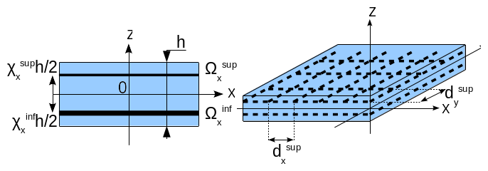
Figure 3-a: Section of the reinforced concrete slab; perspective view.

The dimensionless positions of the reinforcing plies in the thickness verify:

\({\chi }_{x\mathrm{/}y}^{\text{sup}}\mathrm{\in }\mathrm{]}\mathrm{0,1}\mathrm{[}\) and \({\chi }_{x\mathrm{/}y}^{\text{inf}}\mathrm{\in }\mathrm{]}\mathrm{-}\mathrm{1,0}\mathrm{[}\)

The equivalent density of the reinforced concrete plate is defined by a simple average weighted by the densities \({\rho }_{a}\), \({\rho }_{b}\) of the respective proportions of the two materials (law of mixtures). It is used to establish the kinetic energy of the plate.

(3.19)\[ {\ rho} _ {\ mathit {eq}}\ mathrm {=} {\ rho} _ {b} +\ frac {{\ rho} _ {a}} {h} ({\ Omega} _ {eq} _ {x}} _ {x}} ^ {\ text {eq}}} {h} ({\ omega} _ {x}} {h}} ({\ omega} _ {x}} {h}} ({\ omega} _ {x}} {h}} ({\ omega} _ {x}} _ {y}} ^ {\ omega} _ {y}} ^ {\ text {sup}} ^ {\ text {sup}}} ^ {\ omega} _ {y} ^ {\ sub}} ^ {\ omega} _ {y} ^ text {sup}} + {\ omega} _ {y} ^ {\ text {inf}})\]

This equivalent density must be entered under the keyword ELAS of the DEFI_MATERIAU operator for defining the concrete material, with the Young’s modulus and the Poisson’s ratio of concrete. This last data is used to establish an estimate of the speed of the waves, used to control the time step in explicit integration (Current condition):

	E	NUDE	RHO
parameter	\({E}_{b}\)	\({\nu }_{b}\)	\({\rho }_{\mathit{éq}}\)
SI units	[Pa]	without	[kg/m3]

3.1. Identification of linear elastic behavior parameters

The linear elastic behavior is a priori orthotropic and integrates a membrane—flexure coupling. To perform an elastic calculation prior to a nonlinear analysis, we want to represent this type of behavior of the reinforced concrete structure as best as possible.

It is proposed to identify the coefficients of linear elastic behavior in two ways:

by**the orthotropic approach* where the elastic membrane-flexure matrix is constructed from the elastic characteristics of concrete (\({E}_{b}\), \({\nu }_{b}\)), steel (\({E}_{a}\)) and the geometric characteristics of the reinforced concrete section, cf. ().

by**the isotropic approach* where the elastic parameters of the equivalent homogenized medium are determined.

The global elastic law of the reinforced concrete slab with membrane coupling and flexure is written with the tensors \({H}_{m}\), \({H}_{f}\), \({H}_{\mathit{mf}}\) and is given in the orthogonal local coordinate system linked to the reinforcement by:

(3.19)\[\begin{split} (\ begin {array} {c} {N}} _ {\ mathit {xx}} {\ mathit {xx}}}\\ {array}}\\ {\ mathrm {2N}} _ {\ mathit {xy}}}\\ {xy}}}\\ {xy}} _ {\ mathit {xy}}} _ {\ mathit {xy}}} _ {\ mathit {xy}}} _ {\ mathit {xy}}} _ {\ mathit {xy}}} _ {\ mathit {xy}}} _ {\ mathit {xy}}} _ {\ mathit {xy}}} _ {\ mathit {xy}}} _ {\ mathit {xy}}} _ {\ mathit {xy}}} _ {\ mathit {xy}} _ {\ mathit {xy}}\ end {array})\ mathrm {=})\ mathrm {=} (\ begin {array} {ccc} {H} _ {1111} ^ {m} & {H} & {H} & {H} & {H} & {H} & {H} _ {2222} {m} & {H} _ {2222} {m} & {2222} ^ {m} & {H} _ {2222} {m} & {H} _ {2222} {m} & {H} _ {2222} {m} & {H} _ {2222} {m} & {H}} _ {2222} {m} & {H} _ {2222} {m} & {H} _ {2222} {m} & 0\\ 0& 0& {H} _ {1212} _ {1212} ^ {1212} ^ {1212} ^ {H} _ {1111} ^ {\ mathit {mf}}} & {H}} _ {1212} ^ {1122} ^ {1122}} ^ {H} _ {1122} ^ {\ mathit {mf}}} & {{1122}} ^ {\ mathit {mf}}} & {H} _ {2222} ^ {\ mathit {mf}}} & 0\\ 0& 0\\ 0& 0& {H} _ {1212} ^ {\ mathit {mf}}\ end {array})\\ (\ begin {array} {{array} {{array}} {{ccc}} {ccc}} {H}} _ {array})\\ (\ begin {array}} {{array}})\\ (\ begin {array}} {{array}} {{array}})\\ (\ begin {array}} {{array}} {{ccc}} {H}} _ {1122}) ^ {\ mathit {mf}} ^ {\ mathit {mf}} ^ {\ mathit {mf}}} & {H} _ {1122 0\\ {H} _ {1122} ^ {\ mathit {mf}}} & {H} _ {2222} ^ {\ mathit {mf}}} & 0\\ 0& {H} _ {1212} _ {1212} ^ {1212} ^ {1212} ^ {1212} ^ {1212} ^ {1212} ^ {1212} ^ {12} ^ {1212} ^ {1212} ^ {1212} ^ {1212} ^ {1212} ^ {1212} ^ {1212} ^ {1212} ^ {1212} ^ {1212} ^ {1212} ^ {1212} ^ {1212} ^ {1212} ^ {MF} ^ {MF}} ^ {MF}} ^ {F} ^ {F} ^ {F} ^ {1122} ^ {f} & 0\\ {H} _ {1122} _ {1122} ^ {H}} _ {2222} ^ {f} & 0\ 0& {H} _ {1212} _ {1212} ^ {f} ^ {f}\ {f}\\\\\\ {f}\\\\ {f} _ {1212} ^ {f} ^ {f} _ {1212} ^ {f} ^ {f}}\ {f} _ {1212} ^ {f} ^ {f} _ {f} {f}\ {f} _ {1212} ^ {f}}\ {f} _ {1212} ^ {f} {f} _ {1212} ^ {f}} {f} _ {1212} ^ {f} ^ {f}\ epsilon} _ {\ mathit {yy}}}\\ 2 {\ epsilon}} _ {\ mathit {xy}}\\ {\ kappa} _ {\ mathit {xx}}\\ {\ kappa}}\\ {\ kappa} _ {\ mathit {\ kappa}} _ {\ mathit {xy}}}\\ {\ kappa}}\\ {\ kappa}}\\ {\ kappa}}\\ {\ kappa} _ {\ mathit {xx}}\\ {\ kappa}}\\ {\ kappa}}\\ {\ kappa} _ {\ mathit {xx}}\\ {\ kappa}}\\ {\ kappa}} _\end{split}\]

The orthogonal local coordinate system linked to the reinforcement is defined with AFFE_CARA_ELEM (keyword factor COQUE, keyword ANGL_REP).

In this expression, \({H}_{\mathit{ijkl}}^{m}\) are membrane stiffness, \({H}_{\mathit{ijkl}}^{f}\) are flexure stiffness, and \({H}_{\mathit{ijkl}}^{\mathit{mf}}\) are membrane-flex coupling stiffness. Orthotropy requires that the terms \({H}_{\mathit{ij}12}\) be zero in this frame of reference. In the case of two symmetric reinforcement grids, membrane-flexure decoupling is obtained: \({H}_{\mathit{ijkl}}^{\mathit{mf}}\mathrm{=}0\).

We check that it is necessary to check: \({H}_{1111}^{m}{H}_{1111}^{f}\mathrm{-}{({H}_{1111}^{\mathit{mf}})}^{2}>0\), in the same direction as in the other direction. In the same way we must have: \({H}_{1111}^{m}{H}_{2222}^{m}\mathrm{-}{({H}_{1212}^{m})}^{2}>0\), \({H}_{1111}^{f}{H}_{2222}^{f}\mathrm{-}{({H}_{1212}^{f})}^{2}>0\), always because of the definitive-positive nature of the elasticity tensor.

• Orthotropic approach ( not available in Code_Aster now)

The coefficients are constructed directly by the following approximated relationships:

\(\mathrm{\{}\begin{array}{c}{H}_{1111}^{m}\mathrm{=}\frac{{E}_{b}h}{1\mathrm{-}{\nu }_{b}^{2}}+{E}_{a}{\mathrm{\langle }\Omega \mathrm{\rangle }}_{x}\\ {H}_{2222}^{m}\mathrm{=}\frac{{E}_{b}h}{1\mathrm{-}{\nu }_{b}^{2}}+{E}_{a}{\mathrm{\langle }\Omega \mathrm{\rangle }}_{y}\end{array}\), \(\mathrm{\{}\begin{array}{c}{H}_{1122}^{m}\mathrm{=}\frac{{\nu }_{b}{E}_{b}h}{1\mathrm{-}{\nu }_{b}^{2}}\\ {H}_{1212}^{m}\mathrm{=}\frac{{E}_{b}h}{1+{\nu }_{b}}\end{array}\) \(\mathrm{\{}\begin{array}{c}{H}_{1111}^{f}\mathrm{=}\frac{{E}_{b}{h}^{3}}{12(1\mathrm{-}{\nu }_{b}^{2})}+\frac{{E}_{a}{h}^{2}}{4}{\mathrm{\langle }{\chi }^{2}\Omega \mathrm{\rangle }}_{x}\\ {H}_{2222}^{f}\mathrm{=}\frac{{E}_{b}{h}^{3}}{12(1\mathrm{-}{\nu }_{b}^{2})}+\frac{{E}_{a}{h}^{2}}{4}{\mathrm{\langle }{\chi }^{2}\Omega \mathrm{\rangle }}_{y}\end{array}\), \(\mathrm{\{}\begin{array}{c}{H}_{1122}^{f}\mathrm{=}\frac{{\nu }_{b}{E}_{b}{h}^{3}}{12(1\mathrm{-}{\nu }_{b}^{2})}\\ {H}_{1212}^{f}\mathrm{=}\frac{{E}_{b}{h}^{3}}{12(1+{\nu }_{b})}\end{array}\) \(\mathrm{\{}\begin{array}{c}{H}_{1111}^{\mathit{mf}}\mathrm{=}\frac{{E}_{a}h}{2}{\mathrm{\langle }\chi \Omega \mathrm{\rangle }}_{x}\\ {H}_{2222}^{\mathit{mf}}\mathrm{=}\frac{{E}_{a}h}{2}{\mathrm{\langle }\chi \Omega \mathrm{\rangle }}_{y}\end{array}\), \(\mathrm{\{}\begin{array}{c}{H}_{1122}^{\mathit{mf}}\mathrm{=}0\\ {H}_{1212}^{\mathit{mf}}\mathrm{=}0\end{array}\) where we put, to simplify, the expressions: \({\mathrm{\langle }\Omega \mathrm{\rangle }}_{x}\mathrm{=}{\Omega }_{x}^{\text{sup}}+{\Omega }_{x}^{\text{inf}}\), \({\mathrm{\langle }\Omega \mathrm{\rangle }}_{y}\mathrm{=}{\Omega }_{y}^{\text{sup}}+{\Omega }_{y}^{\text{inf}}\) \({\mathrm{\langle }\chi \Omega \mathrm{\rangle }}_{y}\mathrm{=}{\chi }_{y}^{\text{sup}}{\Omega }_{y}^{\text{sup}}+{\chi }_{y}^{\text{inf}}{\Omega }_{y}^{\text{inf}}\), \({\mathrm{\langle }\chi \Omega \mathrm{\rangle }}_{y}\mathrm{=}{\chi }_{y}^{\text{sup}}{\Omega }_{y}^{\text{sup}}+{\chi }_{y}^{\text{inf}}{\Omega }_{y}^{\text{inf}}\) \({\mathrm{\langle }{\chi }^{2}\Omega \mathrm{\rangle }}_{x}\mathrm{=}{\chi }_{x}^{{\text{sup}}^{2}}{\Omega }_{x}^{\text{sup}}+{\chi }_{x}^{{\text{inf}}^{2}}{\Omega }_{x}^{\text{inf}}\), \({\mathrm{\langle }{\chi }^{2}\Omega \mathrm{\rangle }}_{x}\mathrm{=}{\chi }_{x}^{{\text{sup}}^{2}}{\Omega }_{x}^{\text{sup}}+{\chi }_{x}^{{\text{inf}}^{2}}{\Omega }_{x}^{\text{inf}}\)

(3.1.2)

It is thus assumed that steels do not provide stiffness in terms of membrane distortion of the plate, or in torsion.

Note:

The orthotropic approach is not available in the current version. It is envisaged to introduce it in the next evolutions of the model.

• Isotropic approach

The global elastic matrix for eq. 3.1.1 is constructed by assuming:

(3.19)\[\begin{split} (\ begin {array} {ccc} {H} _ {1111} _ {1111}} ^ {m} & {H} _ {1122} _ {1122} ^ {m} & {H} & {H} _ {2222}} _ {2222}} _ {2222}} _ {2222}} ^ {H}\ end {array})\ mathrm =}\ frac {{E} _ {\ mathit {eq}}} ^ {eq}}} ^ {2}}} ^ {eq}} ^ {m})} ^ {m})} ^ {m})} ^ {m})}} ^ {2}}}} ^ {2}}} ^ {2}}}} ^ {2}}}} ^ {2}}}} ^ {2}}}} ^ {2}}}} (\ begin {array} {ccc}} 1& {\nu} _ {\ mathit {eq}}} ^ {m}})} ^ {m}))} ^ {2}}})} ^ {2}}}} (\ begin {array} {ccc}} 1& {\nu} _ {\ mathit {\nu} _ {\ mathit {eq}}} ^ {m} & 1& 0\\ 0& 0& 1\ mathrm {-} {\nu} _ {\ mathit {eq}}} ^ {m}\ end {array}) _ {\ mathit {eq}}}} ^ {m}} ^ {m}\ end {array})\end{split}\]

for the membrane part and

(3.19)\[\begin{split} (\ begin {array} {ccc} {H} _ {1111} _ {1111}} ^ {f} & {H} _ {1122} _ {1122} ^ {f} & {H} & {H} & {H} _ {2222}} _ {2222}} _ {2222}} ^ {H} & {H} _ {1212} ^ {f} _ {1122} ^ {f} & {H} _ {1122} ^ {f} & {H} _ {1122} ^ {f} & {H} _ {1122} ^ {f} & {H} _ {1122} ^ {f} & {H} _ {1122} ^ {f} & {H} _ {1122} ^ {f} & {H} _ {1122} ^ {=}\ frac {{E} _ {\ mathit {eq}}} ^ {f} {f} {h} ^ {3}} {12 (1\ mathrm {-} {({\nu} _ {\ mathit {eq}}}}} ^ {eq}}} ^ {f})} ^ {f})}} ^ {2})} (\ begin {array} {ccc} 1& {\nu} _ {\ mathit {eq}} _ {\ mathit {eq}}} ^ {f})} ^ {f})}} ^ {2})} (\ begin {array} {ccc} 1& {\nu} _ {\ mathit {eq}} _ {\ mathit {eq}}} ^ {f} & 0\\ {\nu} _ {\ mathit {eq}}} ^ {f} & 1& 0\\ 0& 0& 1\ mathrm {-} {\nu} _ {\ mathit {eq}} _ {\ mathit {eq}}} ^ {f}\ end {array})\end{split}\]

for the flexure part. The membrane-flexure coupling is also overlooked:

(3.19)\[\begin{split} (\ begin {array} {ccc} {H} _ {1111} _ {1111}} ^ {\ mathit {mf}}} & {\ mathit {mf}}} & 0\\ {H} _ {1122} _ {1122}} ^ {1122}} ^ {\ mathit {mdf}} _ {2222} ^ {\ mathit {mf}}} & 0\\ {H}} & 0\\ {H} _ {F}} & 0\\ {H} _ {H} _ {1212} ^ {\ mathit {mf}}}\ end {array})\ mathrm {=} 0\end{split}\]

In comparison with [éq. 3.1.3] and [éq. 3.1.4], we opt for the following relationships, by preferring the average behavior in the plane and by averaging over the x and y directions, which give the four necessary elastic coefficients, based on the notations [éq 3.1.2]:

(3.19)\[ {\nu} _ {\ mathit {eq}}} ^ {m}} ^ {m}\ mathrm {=} {\nu} _ {b} _ {b} h} {2 {E} _ {b} _ {b} _ {b} _ {b} _ {b} _ {2}) {b} _ {b} _ {2}) {\ mathrm {\ langle}\ Omega\ mathrm {\ rangle}}} _ {x}} + {\ mathrm {\ langle}\ Omega\ mathrm {\ rangle}}} _ {y})}\]

(3.19)\[ {\nu} _ {\ mathit {eq}}} ^ {f}} ^ {f}\ mathrm {=} {\nu} _ {b} _ {b} h} {2 {E} _ {b} _ {b} _ {b} _ {b} _ {b} _ {b} _ {2} _ {b} _ {2}) {\ mathrm {\ langle} {\ chi} ^ {2}\ Omega\ mathrm {\ rangle}} _ {x}} + {\ mathrm {\ langle} {\ chi} ^ {2}\ Omega\ mathrm {\ rangle}} _ {y})}\]

(3.19)\[\begin{split} {E} _ {\ mathit {eq}}} ^ {m}\ mathrm {=} {E} _ {b}\ frac {{\nu} _ {b} (1\ mathrm {-}} {({\nu}} {({\nu}} _ {\\nu}} _ {\ mathit {eq}} _ {\ mathit {eq}} _ {\ mathit {eq}} _ {\ mathit {eq}} _ {\ mathit {eq}} ^ {m} (1\ mathrm {-} {-} {\nu} _ {b} ^ {2})}\end{split}\]

Of the two elastic approaches, only the second (ii) is currently available.

The elastic coefficients of concrete (\({E}_{b}\), \({\nu }_{b}\)) as well as those of steels \({E}_{a}\) are entered under the keyword ELAS of DEFI_MATERIAU. The characteristics of the arrangement of the steels in the concrete plate (\({\Omega }_{x}^{\text{inf}}\), \({\Omega }_{x}^{\text{sup}}\),,, \({\Omega }_{y}^{\text{inf}}\),,, \({\Omega }_{y}^{\text{sup}}\), \({\chi }_{x}^{\text{inf}}\),, \({\chi }_{x}^{\text{sup}}\), \({\chi }_{y}^{\text{inf}}\), \({\chi }_{y}^{\text{sup}}\)) are given under the keyword NAPPE of DEFI_GLRC.

The height \(h\) of the section is also provided by the operator DEFI_GLRC, keyword BETON, operand EPAIS. The directions of the local orthotropy coordinate system are defined by the operator AFFE_CARA_ELEM, keyword COQUE with the operand ANGL_REP. The linear elastic behavior can be used in nonlinear analysis under the keyword COMPORTEMENT with the operand RELATION = “GLRC_DAMAGE”.

3.2. Identification of parameters of damageable elasto-plastic behavior

The damage model, [§2.3], is formulated under the assumption of isotropy (see [§3.1, ii]), which is a reasonable approximation in most cases. In addition, it is accepted that the flexion-membrane coupling (terms \({H}_{\mathit{ijkl}}^{\mathit{mf}}\)) in the elastic phase of the behavior is negligible.

According to [§3.1, ii] we identify the flexion-membrane elasticity tensor (cf. the tensors \({H}_{m}\) and \({H}_{f}\) defined by [éq 2.3.3] and [éq. 2.3.4]):

(3.19)\[\begin{split} (\ begin {array} {c} {N}} _ {\ mathit {xx}} {\ mathit {xx}}}\\ {array}}\\ {\ mathrm {2N}} _ {\ mathit {xy}}}\\ {xy}}}\\ {xy}} _ {\ mathit {xy}}} _ {\ mathit {xy}}} _ {\ mathit {xy}}} _ {\ mathit {xy}}} _ {\ mathit {xy}}} _ {\ mathit {xy}}} _ {\ mathit {xy}}} _ {\ mathit {xy}}} _ {\ mathit {xy}}} _ {\ mathit {xy}}} _ {\ mathit {xy}}} _ {\ mathit {xy}} _ {\ mathit {xy}}\ end {array})\ mathrm {=})\ mathrm {=} (\ begin {array} {cc}\ frac {{e}} _ {\ mathit {eq}}} ^ {m}}} ^ {m}}} ^ {m}} ^ {m}}} ^ {m}}} ^ {m}} ^ {m}}} ^ {m} h} {1\ mathrm} h} {1\ mathrm {-}} {1\ mathrm {-}} {-} {-} {({\nu}} _ {\ mathit {eq}})} ^ {2}}} (\ begin {array}})} ^ {2}}} (\ begin {array}}} {ccc} 1& {\nu} _ {\ mathit {eq}}} ^ {m}} ^ {m} & 0\\ {\nu} _ {\ mathit {eq}} ^ {m} & 1& 0\\ 0& 0& 0& 0& 1\ mathrm {-} {\ m}\ end {array}) & (0)\ 0& 0& 0& 0& 1\\ 0& 0& 1\ mathrm {-} {\nu} _ {\ mathit {eq}} ^ {m} ^ {m} & 1& 0\\ 0& 0& 0& 0& 0& 0& 1\\ 0& 0& 0& 1\ mathrm {-} {\nu} _ {\ mathit {eq}}} ^ {m} ^ {(0) &\ frac {{E} _ {\ mathit {eq}}} ^ {f} {f} {h} ^ {3}} {12 (1\ mathrm {-} {({\nu}} _ {\ mathit {eq}}}}} ^ {eq}}} ^ {f}})} ^ {2})} {\ mathrm {-} {\ u} {\ u} _ {\ mathit {eq}}} ^ {f})}} ^ {2})} (\ begin {array} {ccc} 1& {\nu} _ {\ mathit {eq}} _ {\ mathit {eq}}}} ^ {f})} ^ {2})} (\ begin {array} {ccc} 1& {q}} ^ {f} & 0\\ {\nu} _ {\ mathit {eq}} ^ {f} & 1& 0\\ 0& 0& 0& 1\ mathrm {-} {\nu} _ {\ mathit {eq}} ^ {f}\ end {array})\ end {array})\ end {array}}) (\ end {array}}) (\ end {array}})\ end {array})) (\ begin {array})) (\ begin {array})) (\ begin {array})) (\ begin {array})) (\ begin {array})) (\ begin {array})) (\ begin {array})) (\ begin {array})) (\ begin {array})) (\ begin {array})) (\ begin {array})) (\ begin {array})) (\ begin {array} yy}}\\ 2 {\ epsilon} _ {\ mathit {xy}}\\ mathit {xy}}}\\ {\ kappa}} _ {\ mathit {yy}} _ {\ mathit {yy}}}\\\ 2 {\ kappa}}\\ 2 {\ kappa}} _ {\ mathit {xy}}}\\ {\ kappa}} _ {\ mathit {yy}} _ {\ mathit {yy}}} _ {\ mathit {yy}}} _ {\ mathit {yy}}} _ {\ mathit {yy}}} _ {\ mathit {yy}}}\end{split}\]

3.2.1. Identification of damage thresholds

The damage thresholds defined by [éq. 2.4.3] must be identified from the crack limits in pure mono-axial tension and in pure mono-axial bending (in the positive \({M}_{1}^{d}\) and negative \({M}_{2}^{d}\) directions) of the reinforced concrete slab, which are themselves defined from the tensile strength threshold of concrete \({\sigma }_{\mathit{ft}}\mathrm{\ge }0\) (cf. [bib2]). To do this, the analytical resolution of the case of a reinforced concrete beam is used in the same way as the slab. The approximation consisting in considering reinforcement layers averaged in the directions \(x\) and \(y\) is retained. So we will admit that we have \({H}_{1111}^{m}\mathrm{\equiv }{H}_{2222}^{m}\), \({H}_{1111}^{f}\mathrm{\equiv }{H}_{2222}^{f}\) and \({H}_{1111}^{\mathit{mf}}\mathrm{\equiv }{H}_{2222}^{\mathit{mf}}\). Not taking this approximation into account leads to cumbersome and unnecessary calculations.

In pure positive mono-axial flexure \({M}_{\mathit{xx}}\), with \({N}_{\mathit{xx}}\mathrm{=}0\), \({\epsilon }_{\alpha y}\mathrm{=}0\), \({\kappa }_{\mathit{xy}}\mathrm{=}0\) and \({\kappa }_{\mathit{yy}}\mathrm{=}\mathrm{-}{\nu }_{\mathit{éq}}^{f}{\kappa }_{\mathit{xx}}\), \(\alpha \mathrm{=}\mathrm{\{}x,y\mathrm{\}}\), with,, and,, concrete damage is first achieved in the lower skin of the reinforced concrete slab: \({\sigma }_{\mathit{ft}}\mathrm{=}\frac{{E}_{b}}{1\mathrm{-}{\nu }_{b}^{2}}({\epsilon }_{\mathit{xx}}+{\kappa }_{\mathit{xx}}h\mathrm{/}2)\). We therefore have the following relationships, cf. [éq. 3.1.2], [éq. 3.1.3] and [éq. 3.1.4]:

\({\epsilon }_{\mathit{xx}}\mathrm{=}\mathrm{-}\frac{{H}_{1111}^{\mathit{mf}}}{{H}_{1111}^{m}}{\kappa }_{\mathit{xx}}\)

then

(3.19)\[\begin{split} \ begin {array} {ccc} {M} _ {\ mathit {xx}} _ {\ mathit {xx}}} &\ mathrm {=} & ({H} _ {f}\ mathrm {-} {H} {H} _ {1122} _ {1122}} ^ {h} _ {\ mathit {eq}}} ^ {f}\ mathrm {-} {H}\ mathrm {-} {H} _ {-} {H} _ {1122}} _ {1122}} ^ {H} _ {1111} ^ {\ mathit {mf}})})} {{H}})} {{H} _ {1111} _ {\ mathit {xx}}\\ &\ mathrm {=}} & ({H}}}} & ({H}}} & ({H}} _ {H} _ {H} _ {H} _ {H} _ {H} _ {H} _ {H} _ {H} _ {H} _ {H} _ {H} _ {H} _ {H} _ {H} _ {H} _ {H} _ {H} _ {H} _ {H} _ {H} _ {H} _ {H} _ {H} _ {H} _ {H} _ {H} _ {H} _ {H} _ {H} {f})} ^ {2})\ mathrm {-}\ frac {({H} _ {1111} ^ {\ mathit {mf}})} {{H} _ {1111} _ {1111} ^ {m}}}) {\ kappa}}) {\ kappa}} _ {\ mathit {xx}}\ end {array}}\end{split}\]

(3.19)\[ {\ sigma} _ {\ mathit {ft}}}\ mathrm {=}\ mathrm {=}\ frac {{E} _ {b} {\ kappa} _ {\ mathit {xx}}}} {1\ mathrm {-}} {-}} {1\ mathrm {-}} {1\ mathrm {-}} {-} {frac {-}} {frac {-}} {frac {-}} {frac {-}} {\ frac {-} {-} {\ frac {-}} {\ frac {-} {-} {\ frac {-}} {\ frac {-} {-} {\ frac {H}} {-} {\ frac {H}} _ {11_ 11} ^ {\ mathit {mf}}}} {{H} _ {1111} _ {1111}} ^ {m}})\ mathrm {=}\ frac {{E} _ {b} {M} _ {\ mathit {xx}}}} {\ mathit {xx}}}} {\ mathit {xx}}}} {\ mathit {xx}}}} {\ mathit {xx}}}}} {\ mathit {xx}}}}} {\ mathit {xx}}}}} {1\ mathrm {-} {\ 1111} {x}}}} {1\ mathrm {-} {\nu} _ {b} {H} {M} _ {1111}}} {1111} ^ {m}}} {{}} {(1\ mathrm {-} {-} {({\nu}} _ {\ mathit {eq}}} ^ {f})} ^ {2}) {H} _ {1111} ^ {H} {H} {H} {H} {H} {11}} ^ {H}} {1111} ^ {11} ^ {f})} ^ {f}\ mathrm {-}} {} (\ frac {h} {2}\ mathrm {-}\ frac {{H} _ {1111} ^ {\ mathit {mf}}}} {{H} _ {1111}} ^ {m}})\]

from where:

(3.19)\[ {M} _ {1} ^ {d}\ mathrm {=} (1\ mathrm {-} {\nu} _ {b} ^ {2})\ frac {{\ sigma} _ {\ mathit {ft}}} {\ mathit {ft}}}}}} {{E}}} {{E} _ {e} _ {e} _ {e} _ {e} _ {e} _ {e} _ {e} _ {b}}}\ frac {-} {({\nu}} _ {\ mathit {ft}}}}} {{E} _ {e} _ {eq}}} ^ {f})} ^ {2}) {H}) {H} _ {1111} _ {1111} ^ {2})} {H}\ mathrm {-} {({H} _ {1111}) ^ {\ mathit {1111}} ^ {11}}} {{H}} {(\ frac {h}} {1111}}} {(\ frac {h}} {1111}}} {(\ frac {h}} {1111}} ^ {11}}} {(\ frac {h}} {1111}} ^ {11}}} {(\ frac {h}} {1111}}) ^ {11}} {mathrm {-}\ frac {{H} _ {1111} _ {1111}} ^ {\ mathit {mf}}}} {{H} _ {1111} ^ {m}})})}} ^ {\ mathrm {-} 1})} ^ {\ mathrm {-} 1}\]

In the case where we neglect the flexion-membrane coupling, \({H}_{1111}^{\mathit{mf}}\mathrm{=}0\), we simply have:

(3.19)\[ {M} _ {1} ^ {d}\ mathrm {=}\ mathrm {=}}\ frac {{\ sigma} _ {\ mathit {ft}}} {h} ^ {2}} {6}\ frac {{\nu}} _ {{b}} _ {{b}}} {b}}} {b}}} {b}}} {b}}} {b}}} {b}}} {b}}} {b}}} {b}}} {b}}} {b}}} {b}}} {b}}} {b}}} {b}}} {b}}} {b}}} {b}}} {b}}} {b}}} {b}}} {b}}} {b}} {\ mathit {eq}} ^ {f})} ^ {2})\]

Likewise, in pure negative mono-axial bending \({M}_{\mathit{xx}}\), with \({N}_{\mathit{xx}}\mathrm{=}0\), \({\epsilon }_{\alpha y}\mathrm{=}0\), \({\kappa }_{\mathit{xy}}\mathrm{=}0\) and, \({\kappa }_{\mathit{yy}}\mathrm{=}\mathrm{-}{\nu }_{\mathit{éq}}^{f}{\kappa }_{\mathit{xx}}\), \(\alpha \mathrm{=}\mathrm{\{}x,y\mathrm{\}}\), with,, and,,, concrete damage is first achieved in the upper skin of the reinforced concrete slab: \({\sigma }_{\mathit{ft}}\mathrm{=}\frac{{E}_{b}}{1\mathrm{-}{\nu }_{b}^{2}}({\epsilon }_{\mathit{xx}}\mathrm{-}{\kappa }_{\mathit{xx}}h\mathrm{/}2)\). We therefore have the following relationships:

(3.19)\[ {\ sigma} _ {\ mathit {ft}}}\ mathrm {=}\ mathrm {=}\ mathrm {-}\ frac {{E} _ {\ kappa}} _ {\ mathit {xx}}}} {\ mathrm {xx}}}}} {1\ mathrm {-}}} {1\ mathrm {-}} {\ frac {-} {frac}} {{H} _ {1111} ^ {\ mathit {mf}}}} {{H} _ {1111} ^ {m}})\ mathrm {=}\ mathrm {-}\ frac {{E}\ frac {{E} _ {b} _ {b} {b} {b} {b} {b} {e} _ {b}} _ {b} {E} _ {b} {e} _ {b} {e} _ {b} {e} _ {b} {e} _ {b} {e} _ {b} {e} _ {b} {e} _ {b} {e} _ {b} {e} _ {b} {e} _ {b} {e} _ {b} {e} _ {b} {e} _ {frac {{H} _ {1111} ^ {m}}} {(1\ mathrm {-}} {({\nu} _ {\ mathit {eq}} ^ {f})} ^ {2}) {H}) {H}) {H}}} {H}}} {(H} _ {1111} ^ {H}}) {H} _ {1111} ^ {\ mathit {mf}})} ^ {2}}} (\ frac {h} {2}} +\ frac {{H} _ {1111} ^ {\ mathit {mf}}}}} {{H}}} {{H}} _ {1111} ^ {m}})\]

from where:

(3.19)\[ {M} _ {2} ^ {d}\ mathrm {=}\ mathrm {=}\ mathrm {-} {-} {\nu} _ {b} ^ {2})\ frac {{\ sigma} _ {\ sigma} _ {sigma} _ {\ sigma} _ {\ sigma} _ {\ sigma} _ {\ sigma} _ {\ mathit {eq}} ^ {f})}} ^ {2})} ^ {2}) {H} _ {1111} ^ {f}\ mathrm {-} {({H}) {({H} _ {H} _ {2}}) {\ mathit {2}} {{f}}\ mathrm {-}} {-} {{m}} {(H}} {H}} {-} {m}} {m}} {m}} {(\ frac) {h} {2} +\ frac {{H} _ {1111} _ {1111} _ {{H}} _ {1111} ^ {m}})})}} ^ {\ mathrm {-} 1})} ^ {\ mathrm {-} 1}\]

In the case where the flexion-membrane coupling is neglected, we simply have:

(3.19)\[ {M} _ {1} ^ {d}\ mathrm {=}\ mathrm {=}\ mathrm {-}\ frac {{\ sigma} _ {\ mathit {ft}} {h} ^ {2}} {6}} {6}} {6}\ frac {{\nu}}\ frac {{\nu}} _ {\ mathit {eq}}} {h} ^ {2}}} {6}} {6}\ frac {{\nu} _ {b}} {b}} {{b}} {b}} {{\nu} _ {\ mathit {eq}} ^ {f}}} {6}} {6}\ frac {{\nu} _ {b}} {b}} {{\nu} _ {{({\nu} _ {\ mathit {eq}}} ^ {f})} ^ {2})\]

Note:

We check that: \({M}_{1}^{d}\mathrm{\ge }0\) and \({M}_{2}^{d}\mathrm{\le }0\).

All that remains is to connect these moments of cracking to the thresholds \({k}_{1}\), \({k}_{2}\) defined in [éq. 2.5.3]. Since the load is being performed from a blank state, \({d}_{1}\mathrm{=}{d}_{2}\mathrm{=}0\). Hence the forces of damage (energy return), cf. [éq. 2.4.3]:

\({Y}_{j}\mathrm{=}\frac{1\mathrm{-}\gamma }{{(1+{d}_{j})}^{2}}(\frac{{\lambda }_{f}}{2}\mathit{tr}{({\kappa }^{e})}^{2}H({(\mathrm{-}1)}^{j}\mathit{tr}({\kappa }^{e}))+{\mu }_{f}\mathrm{\sum }_{i}{({\tilde{\kappa }}_{i}^{e})}^{2}H({(\mathrm{-}1)}^{j}{\tilde{\kappa }}_{i}^{e}))\)

where we apply \({d}_{j}\mathrm{=}0\), \({\kappa }^{p}\mathrm{=}0\), \({\kappa }^{e}\mathrm{=}\kappa\), \({\kappa }_{\mathit{xy}}\mathrm{=}0\) and \({\kappa }_{\mathit{yy}}\mathrm{=}\mathrm{-}{\nu }_{\mathit{éq}}^{f}{\kappa }_{\mathit{xx}}\) in order to obtain:

\({Y}_{j}\mathrm{=}\frac{1}{2}(1\mathrm{-}\gamma )({\lambda }_{f}{(1\mathrm{-}{\nu }_{\mathit{éq}}^{f})}^{2}+{\mu }_{f}){\kappa }_{\mathit{xx}}^{2}\)

Using [éq. 3.1.1] from the [R7.01.32] document:

\({\lambda }_{f}\mathrm{=}\frac{{h}^{3}{\nu }_{f}{E}_{\mathit{éq}}^{f}}{12(1\mathrm{-}{\nu }_{f}^{2})}\), \({\mu }_{f}\mathrm{=}\frac{{h}^{3}{E}_{\mathit{éq}}^{f}}{24(1+{\nu }_{f})}\)

we get:

\(\begin{array}{ccc}{Y}_{j}& \mathrm{=}& \frac{{h}^{3}}{24}(1\mathrm{-}\gamma ){E}_{\mathit{éq}}^{f}\frac{1+{\nu }_{\mathit{éq}}^{f}(1\mathrm{-}{\nu }_{\mathit{éq}}^{f})}{1+{\nu }_{\mathit{éq}}^{f}}{\kappa }_{\mathit{xx}}^{2}\\ & \mathrm{=}& \frac{{h}^{3}}{24}(1\mathrm{-}\gamma ){E}_{\mathit{éq}}^{f}\frac{1+{\nu }_{\mathit{éq}}^{f}(1\mathrm{-}{\nu }_{\mathit{éq}}^{f})}{1+{\nu }_{\mathit{éq}}^{f}}{(\frac{{M}_{\mathit{xx}}}{{H}_{1111}^{f}(1\mathrm{-}{({\nu }_{\mathit{éq}}^{f})}^{2})})}^{2}\\ & \mathrm{=}& \frac{{h}^{3}}{24}(1\mathrm{-}\gamma ){E}_{\mathit{éq}}^{f}\frac{1+{\nu }_{\mathit{éq}}^{f}(1\mathrm{-}{\nu }_{\mathit{éq}}^{f})}{1+{\nu }_{\mathit{éq}}^{f}}{(\frac{12}{{E}_{\mathit{éq}}^{f}{h}^{3}}{M}_{\mathit{xx}})}^{2}\\ & \mathrm{=}& \frac{6}{{h}^{3}}\frac{(1\mathrm{-}\gamma )}{{E}_{\mathit{éq}}^{f}}\frac{1+{\nu }_{\mathit{éq}}^{f}(1\mathrm{-}{\nu }_{\mathit{éq}}^{f})}{1+{\nu }_{\mathit{éq}}^{f}}{M}_{\mathit{xx}}^{2}\end{array}\)

then:

(3.19)\[ {k} _ {1}\ mathrm {=}\ frac {6} {6} {6} {{h}} ^ {3}}\ frac {(1\ mathrm {-}\ gamma)} {{E} _ {\ mathit {eq}} _ {\ mathit {eq}} _ {\ mathit {eq}} _ {\ mathit {eq}} _ {\ mathit {eq}} _ {\ mathit {eq}} _ {\ mathit {eq}} _ {\ mathit {eq}} _ {\ mathit {eq}} _ {\ mathit {eq}} _ {\ mathit {eq}} _ {\ mathit {eq}} _ {\ mathit {eq}} {f}} {-} {\nu} _ {\ mathit {eq}}} ^ {f})} {1+ {\nu} _ {\ mathit {eq}} ^ {f}}} {({M}}} {({M} _ {1} _ {1} ^ {d})} ^ {2}\]

The SI units of these thresholds are Joule.

Damaging linear elastic behavior can be used in nonlinear analysis under the keyword COMPORTEMENT with the operand RELATION = “GLRC_DAMAGE”. The DEFI_MATERIAU MF1 and MF2 operator parameters correspond to \({M}_{1}^{d}\) and \({M}_{2}^{d}\).

3.2.2. Identification of the flexural damage slope

According to the relationships developed in [§3.2] of [R7.01.32], the damaging slope is proportional to the parameter \(\gamma\):

(3.19)\[ {p} _ {f}\ mathrm {=}\ gamma {p} _ {\ mathit {alas}}\]

The \(\gamma\) parameter corresponds to the GAMMA parameter entered in the DEFI_GLRC operator.

3.2.3. Identifying the maximum level of flexural damage

In [éq. 2.3.1], it was planned to limit the level of flexural damage to the reinforced concrete plate, using values of \({d}_{j}^{\mathit{max}}\). These values are associated with the moment-curvature slopes, for the two loading directions \(j\mathrm{=}\mathrm{1,2}\), and with respect to the elastic slope, see also []:

\(\frac{{p}_{\mathrm{2,}j}}{{p}_{\mathit{élas}}}\mathrm{=}\frac{1+\gamma {d}_{j}^{\mathit{max}}}{1+{d}_{j}^{\mathit{max}}}\)

Hence, for \(j\mathrm{=}\mathrm{1,2}\):

(3.19)\[ {d} _ {j} ^ {\ mathit {max}}\ mathrm {=}\ frac {{p} _ {\ mathit {alas}}\ mathrm {-} {p} _ {\ mathrm {2,} j}} {\ mathrm {2,} j}} {\ mathrm {-} {p}} _ {f}}\]

In the operator DEFI_GLRC we enter QP1 and QP2 for \({p}_{\mathrm{2,1}}\) and \({p}_{\mathrm{2,2}}\).

3.2.4. Identification of plastic behavior parameters

For elastic and damaged behaviors, it is possible to obtain parameter values analytically from the material and geometric properties of reinforced concrete. To characterize the parameters of plastic behavior, it is imperative to refer to finer modeling (multi-fiber beam, multi-layer or 3D shell). A software of the MOCO type (see [bib10]) is recommended for the automatic identification of GLRC models. Ultimately, it is expected that such a tool will be integrated into Code_Aster. In the current version, the identification of the elasto-plastic part is completely left to the users.

For identification, it is more reasonable to identify the parameters of non-linear behavior from tests, numerical or experimental, with a monotonic loading. For example, you can use a test with homogeneous curvatures and bending moments. Such a test is pseudo-one-dimensional and can be fully represented with a single graph, on which one can identify the damage and plasticity thresholds as well as the slopes corresponding to the various loading phases, see. To measure the effect of membrane stress, the monotonic flexure test must be combined with membrane loading.

Figure 3.2.4-a : Monotonous uniaxial bending.

On the, five phases are distinguished:

1. elastic phase characterized by the slope \({p}_{\mathit{élas}}\)

2. phase corresponding to the damage of the concrete (slope \({p}_{f}\)),

3. recovery of stiffness due to steels after reaching maximum damage (slope \({p}_{2}\))

4. plasticization of steels (slope \({p}_{p}\)).

5. elastic discharge: the discharge slope value is in the range \(\mathrm{[}{p}_{\mathit{élas}},{p}_{f}\mathrm{]}\) for phases i) to iii) and is \({p}_{2}\) for phase iv).

To describe plastic behavior it is necessary to fill in the functions \({M}_{\mathit{jx}}^{p}({N}_{\mathit{xx}}\mathrm{-}{X}_{\mathit{xx}}^{m})\) and \({M}_{\mathit{jy}}^{p}({N}_{\mathit{yy}}\mathrm{-}{X}_{\mathit{yy}}^{m})\), \(j\mathrm{=}\mathrm{1,2}\), as « aster » functions, FMEX1, FMEX2, FMEY1, FMEY2 in DEFI_GLRC. It is recommended to define symbolic functions using the FORMULE command, which should then be transformed into discretized functions using the CALC_FONC_INTERP command. In addition to these functions, one must also enter their first and second derivatives, which, on the other hand, can be calculated by the operator CALC_FONCTION. Typically, these are functions similar to parabolic functions. For a given direction, say \(x\), the two functions \({M}_{\mathrm{1x}}^{p}\) and \({M}_{\mathrm{2x}}^{p}\) define the elastic domain, as in the.

Figure 3.2.4-b :: ** The elastic domain is located between the two flexing moment/membrane effort curves. The graph shows a comparison between the thresholds used by the model GLRC_DAMAGEet those obtained by a multi-layer calculation on the case of a beam.