4. Digital integration#
4.1. Initialization#
In order to perform a calculation using the two damage thresholds, it is necessary to define a set of parameters beforehand. The parameters characterizing the material are as follows: Young’s modulus \(E\), Poisson’s ratio \(\nu\), Poisson’s ratio, toughness \({K}_{\mathrm{Ic}}\), Weibull’s modulus \(m\), characteristic length \({l}_{c}\), and a nominal priming stress at the characteristic length scale. The nominal priming stress at the scale of the characteristic length is introduced in place of the scale factor. It can be expressed by:
: label: eq-4
{sigma} _ {{l} _ {c}}} =frac {{sigma} _ {0} ^ {m}} {{({lambda} _ {0} {l} {l} _ {c} {c} ^ {3})}} ^ {1/m}}
With \({\sigma }_{0}^{m}/{\lambda }_{0}\) the scale factor and m the Weibull module. The nominal priming stress at the characteristic length scale \({\sigma }_{{l}_{c}}\) gives us an idea of the order of magnitude of the priming stress of a domain with a size of \({l}_{c}^{3}\) which is possibly made up of several finite elements during a calculation. More precisely, the probability of initiation corresponding to a request for \({\sigma }_{{l}_{c}}\) is approximately 0.63. In addition to the parameters characterizing the material, the thickness of the modelled structure \({E}_{\mathrm{ps}}\) is specified. It is possible to use a variant of the surface Weibull model instead of volume, for which the scale factor unit is MPamm² instead of MPamm3. In this case, it must be specified that the structure has a thickness of \({E}_{\mathrm{ps}}={l}_{c}\). During the initialization phase, the value of the priming threshold is calculated for each element (stored in as an internal variable). As shown in the, the calculation of the priming threshold \({\sigma }_{a}\) is carried out for each finite element and consists of several steps.
For each finite element, we start by calculating the size of elements \({Z}_{\mathrm{el}}\) according to the position of the nodes and the thickness \({E}_{\mathrm{ps}}\). Then, the propagation threshold is calculated using the equation.
*The priming threshold (also an internal variable) is then calculated (equation) with \(P(\mathrm{el})\in [:ref:`0;1 <0;1>\)] a number drawn at random over a uniform probability density. If the condition of coherence of the two thresholds (equation) is not satisfied, we start again after drawing another value for :math:`P(mathit{el}). In order to make the two thresholds consistent, the Weibull distribution is truncated here. Other choices could have been considered; truncation is carried out here for the sake of simplicity. Note that the choice to perform a truncation on the Weibull distribution requires the choice of a realistic characteristic length. In fact, if the characteristic length chosen is inconsistent (*i.e., * low) with the Weibull parameters used, most of the Weibull distribution can be truncated. In this case, the description of the priming is not faithful to the Weibull parameters considered.
Refer to section 4.4.2 for the choice of parameters.
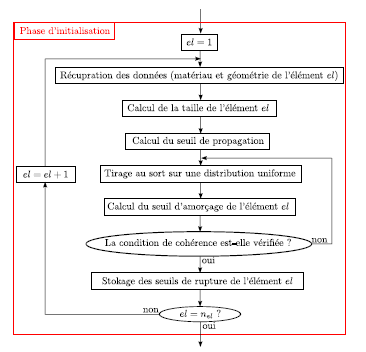
Figure 4.1-a : Calculation initialization scheme
4.2. Solving the global problem#
The global problem concerns the calculation of movements and regularized constraints. The law of behavior that allows stress and damage to be calculated at each Newton’s iteration is implemented according to an implicit scheme. The problem is discretized using the new specific finite elements introduced in the Code_Aster as described in the figure.

Figure 4.2-a : Nodal unknowns of a triangle element
The finite elements used are quadratic in movement and linear in regularized constraints, they therefore comprise 21 degrees of freedom for a triangle element for a plane problem (28 for a quadrangle). Two sets of shape functions and derived shape functions are associated with displacements \(({N}_{u}\mathit{et}{B}_{u})\) and regularized constraints \(({N}_{\stackrel{̄}{\sigma }}\mathit{et}{B}_{\stackrel{̄}{\sigma }})\).
Two equations govern the global problem, one corresponds to classical equilibrium; the other corresponds to the calculation of regularized constraints (for more details on the development of non-local gradient problems, we will refer for example to [R5.04.01]). The integral formulation of the problem is:
: label: eq-4
forall {u} ^ {text {*}}}in {V}}in {V} _ {mathit {ad}} {int} _ {omega}underline {sigma}mathrm {:}\ underline {*}}}in {V}}}in {V}}}in {V}}}in {V} _ {sigma}}mathrm {:}}\underline {*}}}mathrm {:}}\ underline {:}\ underline {*}}}\ underline {*}}}mathrm {:}}\ underline {*}}}mathrm {:}}\ underline {*}}}mathrm {:}}mathrm {.} {T} _ {G}mathit {dG} + {int} + {int} _ {omega} {u} ^ {text {*}}}mathrm {.} {f} _ {V} dOmega
With \({V}_{\mathrm{ad}}\) the space of admissible movements, \({T}_{G}\) the forces imposed on the G edge, the forces imposed on the G edge, \({f}_{V}\) the volume forces and:
: label: eq-4
forallunderline {{s} ^ {text {*}}}}in {[{H} ^ {1} (Omega)]} ^ {6} {int} _ {Omega} _ {Omega} (underline {{s}}} (underline {{s}}}}underline {{s}} ^ {text {*}}}}mathrm {.}} underline {stackrel {!} {sigma}} +nablaunderline {{s} ^ {text {*}}}}mathrm {.}}}mathrm {.} {l} _ {c} ^ {2}underline {stackrel {stackrel {! rel {! rel {sigma}}) domega = {int} _ {omega}underline {{s}} ^ {text {s}} ^ {text {*}}}mathrm {.} underline {sigma} dOmega
In the following part \(\sigma ,\varepsilon \mathrm{et}\stackrel{ˉ}{\sigma }\), we will note the writing of the tensors of the stresses, deformations and regularized constraints in the form of vectors; we denote the displacement vector. The overall resolution comes down to the cancellation of a residue relating to travel that can be written for each of the elements (for more details, we will refer to [R5.03.01]):
: label: eq-4
{F} ^ {u} = {F} _ {text {int}}} + {D} ^ {T}lambda - {F} _ {mathit {ext}} _ {mathit {ext}}
With \({F}_{i}={\int }_{\Omega }{B}_{u}^{T}\sigma d\Omega ,{F}_{e}={\int }_{\Gamma }{N}_{u}^{T}{T}_{g}\mathrm{dG}\) the external load in effort with \({T}_{G}\) the nodal reactions. D is such as \(\mathrm{Du}={u}^{d}\) with \({u}^{d}\) the imposed movements and \(\lambda\) the Lagrange multipliers for conditions at the Dirichlet limits. A residue relating to the regularized stresses is also minimized:
: label: eq-4
{F} ^ {stackrel {459} {sigma}} = {K}}} = {K} ^ {stackrel {459} {sigma}sigma}stackrel {249} {sigma}} - {sigma} - {F} ^ {sigma}
With \({F}^{\sigma }={\int }_{\Omega }{N}_{\stackrel{ˉ}{\sigma }}^{T}\sigma d\Omega \mathrm{et}{K}^{\stackrel{ˉ}{\sigma }\sigma }={\int }_{\Omega }({N}_{\stackrel{ˉ}{\sigma }}^{T}{N}_{\stackrel{ˉ}{\sigma }}+{l}_{c}^{2}{B}_{\stackrel{ˉ}{\sigma }}^{T}{B}_{\stackrel{ˉ}{\sigma }})d\Omega\). In order to minimize the residues presented, the following tangent matrix is used:
: label: eq-4
K=left [begin {array} {cc} {cc}frac {partial {F}} ^ {u}} {partial u} &frac {partial {F} ^ {u}} {partialstackrel {yourself} {stackrel {yourself}} {stackrel {sigma}} {stackrel {sigma}}} {partial u}}} {partial u}}} {partial u}} {sigma}} {partial u}} {sigma}} {partial u}} {sigma}} {partial u}} {sigma}} {partial u}} &sigma}} {partial u}} &sigma}} {partial u}} &sigma}} {partial u} &frac {partial {F} ^ {stackrel {tante} {sigma}}} {partialstackrel {] {sigma}} {sigma}}end {array}right]
With:
: label: eq-4
frac {partial {F} ^ {u}} {partialsigma}} {partial u}} {partial u}}} ^ {T}frac {partialsigma} {partialsigma} {partialsigma} {partialsigma} {partialsigma} {partialepsilon} {partialepsilon} {B} _ {u} domega
: label: eq-4
frac {partial {F} ^ {u}}} {partialstackrel {]} {sigma}} = {int} _ {omega} {B} _ {u} ^ {T}frac {partialsigma}} {partialsigma}} {partialsigma}} {sigma}} {stackrel {yourself} {sigma}} {sigma}} domega
: label: eq-4
frac {partial {F} ^ {stackrel {tante} {sigma}}}} {partialstackrel {tante} {sigma}} = {int} _ {omega} ({N} ({N} _ {N} _ {N} _ {sigma} _ {c}} ^ {T} {N}} _ {sigma}} + {l} _ {c}} + {l} _ {c}} ^ {2} {B} _ {stackrel {tante} {sigma}} ^ {T} {B} _ {stackrel {tante} {sigma}}) domega
: label: eq-4
frac {partial {F} ^ {stackrel {ounty} {sigma}}} {partial u}} {partial u} = {int} _ {omega} - {N} _ {stackrel {ounty} {sigma} {sigma}}} ^ {sigma}} ^ {T}}frac {partialsigma} {partialsigma} {partialsigma} {partialsigma} {partialsigma} {B} _ {u} domega} {B} _ {u} domega
4.3. Implementation of the law of behavior#
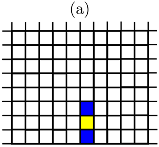
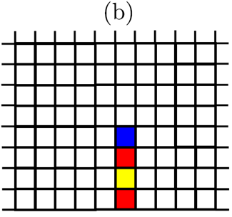
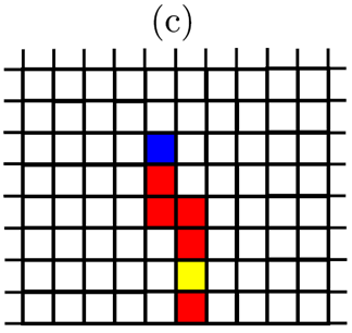
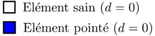
Healthy finite elements (i.e., for which \(d=0\)) can be found in different situations. Either they are at the tip of a crack, in which case they are subject to the propagation threshold, or they are not at the tip of a crack, in which case they are subject to the initiation threshold. Thus, the position of the crack points and their assigned elements are stored during the calculation. The Figure represents the evolution of the state of finite elements during the initiation and propagation of a crack. Initially, if all the finite elements are healthy, they are all subject to their breaking threshold by priming. If a crack occurs in a given element, the element in question is broken (i.e., d=1) and if possible it points to two neighboring elements as shown in Figure (a). At the following Newton iteration, the pointed finite elements are no longer subject to their threshold of rupture by priming but to the threshold of rupture by propagation.
|
|
|
|
||
Figure 4.3-a : States of finite elements
If the pointed finite elements are subjected to such stress that they break, each of them will then, if possible, point to a neighboring finite element which will then be subjected to the threshold of rupture by propagation. As shown in Figure b, if a finite edge element does not find suitable neighboring elements to point to, then nothing happens. Then, the propagation of the initiated crack can continue depending on the level and orientation of the stresses.
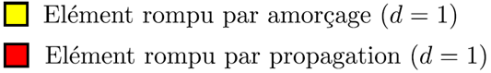
The figure makes it possible to observe more precisely the method of pointing neighboring elements during the priming phase (figure (a)) and during the propagation phase (figure (b)). If in a structural calculation the level of stress reached is sufficient to generate the initiation of a crack in the finite element \({A}_{\mathit{el}}\), then the assumption is made that the crack in question starts at the center of the element and the damage to the finite element in question is equal to \(d=1\). Two crack points \({B}_{\mathit{pt}}\) and \({C}_{\mathit{pt}}\) are then defined, which are the intersections of a line \({\Delta }_{{A}_{\mathit{el}}}\) and the edges of the finite element in question. We define the line \({\Delta }_{{A}_{\mathrm{el}}}\) as passing through the point \({A}_{\mathit{pt}}\) and being perpendicular to the vector \(\overrightarrow{{n}_{{\mathrm{IA}}_{\mathrm{pt}}}}\) which corresponds to the direction associated with the maximum principal regularized stress at the point \({A}_{\mathit{pt}}\) during the break \(\stackrel{̄}{{\sigma }_{{\mathit{IA}}_{\mathit{pt}}}}\). Each of the crack points is then taken care of by a finite element close to the finite element \({A}_{\mathit{el}}\), namely the elements \({B}_{\mathit{el}}\) and \({C}_{\mathit{el}}\). The elements \({B}_{\mathrm{el}}\) and \({C}_{\mathrm{el}}\) are then subject to the threshold of rupture by propagation.
As shown in figure (b), if the propagation threshold is reached at the level of a crack point \({D}_{\mathit{pt}}\) taken over by an element \({D}_{\mathit{el}}\), then the damage to the element \({D}_{\mathrm{el}}\) increases to \(d=1\). The crack tip is then moved along a line \({\Delta }_{{D}_{\mathit{el}}}\) defined as passing through \({D}_{\mathrm{pt}}\) and being perpendicular to \(\vec{{n}_{{\mathit{ID}}_{\mathit{pt}}}}\), the direction associated with the maximum principal regularized stress at point \({D}_{\mathrm{pt}}\) during the rupture \(\stackrel{̄}{{\sigma }_{{\mathit{ID}}_{\mathit{pt}}}}\). The crack point is then positioned at point \({E}_{\mathrm{pt}}\) and taken over by the finite element \({E}_{\mathrm{el}}\). The neighborhood management method developed makes it possible to manage several cracks simultaneously. It also allows each of the defined cracks to bifurcate according to the structural problem as well as according to possible interactions with other cracks of the same structure.
The integration into Code_Aster of the system described is summarized in the figure. In addition, the internal variables used are described in section 4.5.
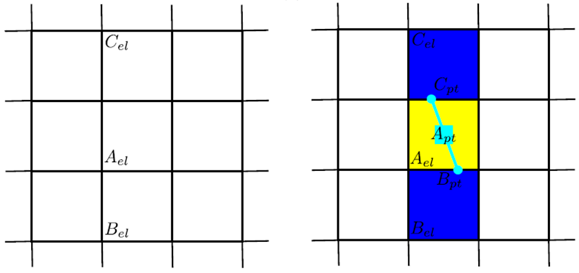
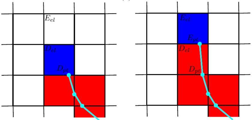
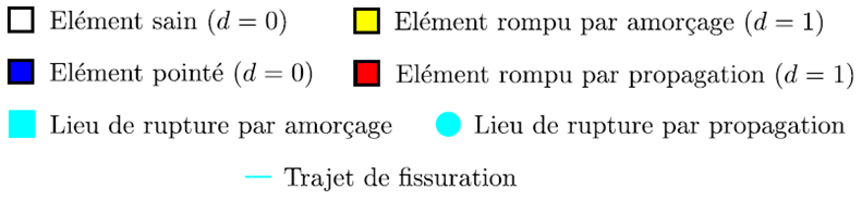
Figure 4.3-b : Identifying neighboring elements
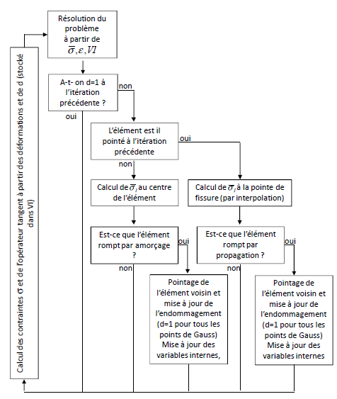
Figure 4.3-c : Integrating priming and propagation thresholds in Code_Aster
The neighborhood management system integration method presented only considers a finite element to be pointed to only if it was pointed during the previous Newton iteration. As a result, each crack point can lead to rupture by propagation of an element by Newtons” iteration. Moreover, the implementation of the material’s behavior is analytical, which guarantees the stability of the converged states. In fact, during a loading step, each crack point can lead to rupture by the propagation of as many elements as necessary to reach equilibrium. As a result, the model presented makes it possible to represent the propagation of macro-cracks even in an unstable phase. Consider the case of a structure subjected to a loading increment containing \({n}_{\mathit{pf}}\) crack points numbered from 1 to \({n}_{\mathit{pf}}\). If during the loading step no new crack starts but each crack tip i must break \({n}_{\mathit{elt}}\) elements in order to reach a steady state, then the number of overall Newton iterations required to solve the problem on the loading increment is \({n}_{\mathit{it}}=\mathit{max}({n}_{\mathit{eli}})\). It can be deduced from this that the duration of the simulations depends very little on the number of cracks present in the structure.
4.4. Material parameters required by law#
4.4.1. Key words#
In summary, 5 material parameters are necessary for the law to be defined in the DEFI_MATERIAU ENDO_HETEROGENE keyword:
WEIBULL: parameter m of the Weibull model,
SY: nominal priming stress,
KI: stress intensity factor \({K}_{i}\),
EPAI: \({E}_{\mathrm{ps}}\) thickness
GR: Seed of the random draw defining the initial faults
The characteristic length is entered under the keyword LONG_CARA from DEFI_MATERIAU.
4.4.2. Identification tips#
The classical Weibull model is based on the weak link hypothesis: the global break in the structure corresponds to the local break, and therefore directly to heterogeneities. The parameters of the Weibull distribution are found experimentally with splitting tests, characterized by an unstable propagation of the first defect which causes the specimen to break suddenly. The weakest link hypothesis is therefore valid in this case. As we have seen, model ENDO_HETEROGENE considers more complex types of cracks, with the formation of a network of cracks. For this reason, the concept of priming was introduced, distinguishing it from propagation; the weak-link hypothesis and the application of the Weibull model in fact stop at the finite element. However, the procedure for experimentally calibrating Weibull parameters by splitting tests is still valid because it is a completely experimental procedure and applies to a case where the weak-link hypothesis is valid; on the other hand, this only corresponds to the initiation of cracking for ENDO_HETEROGENE.
A more complicated step involves determining the remaining parameters: the toughness in \(I\) mode and the characteristic length. Both parameters are used by model ENDO_HETEROGENE to calculate the propagation threshold. The law of fracture mechanics used is non-linear precisely because of the presence of \({l}_{c}\). On the contrary, in experimental tests propagation is associated with tenacity alone, when referring to a linear fracture mechanics model. The two concepts of tenacity used therefore do not seem to coincide, because they are not associated with the same theoretical model. It is therefore necessary to take with care the tenacity values derived from conventional tests.
As far as the characteristic length is concerned alone, this value can be seen as a key to the transition between the small scale, that of the micro defects, to the large scale, that of the macro-cracks. A rule of thumb for choosing it consists in taking a length between the length of the smallest defect and that of a macro-crack. We could therefore make a prior choice of the characteristic length, and then choose the toughness accordingly.
4.5. Description of internal variables#
The model has 12 internal variables that need to be stored at the previous time:
\(\mathrm{VI}(1)\): damage \(d\),
\(\mathit{VI}(2)\): indicator (0 healthy element, 1 pointed element, 2 broken by priming, 3 broken by propagation),
\(\mathrm{VI}(3)\): priming constraint \({\sigma }_{a}\),
\(\mathrm{VI}(4)\): propagation constraint \({\sigma }_{p}\),
\(\mathrm{VI}(5)\): number of the element pointed to number 1,
\(\mathrm{VI}(6)\): number of the element pointed to number 1 if priming,
\(\mathrm{VI}(7)\): breaking Newton’s iteration,
\(\mathrm{VI}(8)\): current Newton’s iteration,
\(\mathrm{VI}(9)\): X coordinate of the crack point (after rupture by propagation),
\(\mathrm{VI}(10)\): Y coordinate of the crack point (after rupture by propagation),
\(\mathrm{VI}(11)\): coordinate \(X\) of the crack point 2 during initiation,
\(\mathrm{VI}(12)\): coordinate \(Y\) of the crack point 2 during initiation,