2. Model description [grimal, 2007]#
2.1. General principle#
The alkali-aggregate reaction and its effects are modelled using a phenomenological approach. This approach takes into account the various important phenomena evolving within concrete and influencing the chemical reaction. The main developments proposed in this model concern the interactions between chemical pressure and, delayed deformations on the one hand and anisotropic deformations induced by the presence of oriented cracks on the other hand.
The effects of humidity on the development of the alkali reaction as well as on the capillary pressure inducing the withdrawal of the matrix are also considered. The dependence between the evolution of the swellings and the state of stress is then a consequence of all these elementary phenomena; the mechanical effects of the alkali-reaction are therefore the consequences of « long-term » internal loading due to the evolution of chemical pressure (\({P}_{g}\) in the figure), combined with external loading \({\sigma }_{i}\).

Figure 2.1-a: Principle of the behavior model of concrete subjected to swelling pressure.
\({P}_{g}\), in addition to the external constraint \({\sigma }_{i}\) stresses the cement matrix. The latter is considered to be a damaging visco-elasto-plastic medium (module VEPD in the figure). The next paragraph shows how the pressure due to gel formation is evaluated, in accordance with the environmental conditions and the state of deformation. Next, the mechanical model is presented in the context of the thermodynamics of irreversible processes.
2.2. Law of evolution of internal pressure#
Pressure \({P}_{g}\) due to gel formation in the porosity is evaluated by assuming that the stress state does not change the chemical progress of the alkali-granulate reaction.
In accordance with the various available models, studied in the bibliographic part [Ulm et al.; Lemarchandet al. ; Coussy, 2002], concrete is considered as a porous medium consisting of a solid matrix and gel occupying part of the connected porosity. This porosity is formed by two types of pores, those initially connected to the reaction sites and those generated by volume deformation modifying the porosity (\({b}^{g}\mathit{tr}(\varepsilon )\) in equation ()).
The porosity connected to the reaction sites is written in the form \({\varphi }_{0}\mathrm{=}{A}_{0}{V}^{g}\), in which, \({A}_{0}\) is the advance from which the initial connected porosity is filled. Thus, as long as the volume of gel created (\({\mathit{AV}}^{g}\)) is less than \({A}_{0}{V}^{g}\), the gel is housed in the connected porosity and \({P}_{g}\) remains zero. \({P}_{g}\) will only increase when all the porosity is filled:
: label: EQ-None
{text {AV}} ^ {g}mathrm {ge}mathrm {ge}mathrm {langle} {A} _ {0} {V} ^ {g} + {b} ^ {g}text {g}text {ge}\ text {ge}\ g}text {ge}\ g}text {tr} (varepsilon)mathrm {rangle}
Taking these remarks into account, an expression relating the gel pressure and the volume of gel created (\({\mathit{AV}}^{g}\)) is proposed:
In this expression:
\({V}_{g}\) is the maximum volume of gel that can be created by the chemical reaction.
\(A\) is the progress of the chemical reaction, increasing from \(0\) for healthy concrete to \(1\) when the reaction is complete.
\({M}_{g}\) can be assimilated to a module of elasticity of the gel and \({b}_{g}\) can be assimilated to a Biot coefficient for the gel.
The various positive parts allow:
taking into account the influence of volume deformation induced by an external loading on a variation in connected porosity,
an increase in chemical pressure if and only if the gel succeeds in filling the connected porosity.
2.3. Progress of the reaction#
The progress of reaction \(A\) mentioned above is a function of the temperature and of the water content of the concrete.
The law of evolution used to assess chemical progress is inspired by the work of S. Poyet [Poyet, 2003]. It shows that the gel created over time (\(t\)) and its creation kinetics are proportional to the degree of saturation (\(\mathit{Sr}\)) of the concrete, the degree of saturation being defined by:
: label: EQ-None
text {Sr}mathrm {=}frac {C} {{C} _ {text {sat}}}}
In this expression, \(C\) is the free water concentration contained per unit volume of concrete and \({C}_{\mathit{sat}}\) is the value of \(C\) when the concrete is fully saturated.
In order to take into account the effect of temperature, Arrhenius’s law is used to model thermal activation [Capra, 1997]. Finally, the following law is proposed:
In this law, \({\mathrm{\alpha }}_{0}\) is a kinetic parameter, \({E}_{a}\) is the activation energy of the alkali-aggregate reaction (usually with a value close to \(47000J\mathrm{/}\mathit{mol}\mathrm{/}°K\) [Lombardi et al., 1995]), \(R\) is the ideal gas constant (\(8.31J\mathrm{/}\mathit{mol}\)), \({T}_{\mathit{ref}}\) (in Kelvin) is the absolute temperature of the test allowing the identification of \({\mathrm{\alpha }}_{0}\) , \(T\) is the temperature of the material point. The term \(\mathrm{\langle }\text{Sr}\mathrm{-}A\mathrm{\rangle }\) means that the chemical affinity of the reaction is conditioned by the degree of saturation of the concrete, Poyet having shown in his thesis that the progress \(A\) (which is a standardized variable) cannot exceed a limit value very close to the degree of saturation, he explains this by the fact that only the fraction of aggregate in contact with water can lead to the reaction. Therefore the amplitude of the reaction is proportional to the degree of saturation \({S}_{r}\).
In the same way, the path taken by the ions to reach reactive silica is all the greater the lower the degree of saturation, which leads to a decrease in kinetics. This kinetic effect of the degree of saturation is taken into account by means of the term \(\frac{⟨\mathit{Sr}-{S}_{r}^{0}⟩}{\left(1-{S}_{r}^{0}\right)}\), in which \({S}_{r}^{0}\) represents the saturation threshold at which the evolution of the chemical reaction becomes possible.
The figure shows some examples of variations in progress \(A\) for different humidity states. The more \({S}_{r}\) is important the bigger \(A\) is, with \(A\) being maximum (\(A=1\)) when the concrete is saturated (\({S}_{r}=1\)). If the concrete remains in an unsaturated state (\({S}_{r}<1\)), the reaction is never complete (\(A<1\)). On the other hand, if the saturation state changes and goes from \(0.6\) to \(1.0\) for example, the progress curve is modified to reach the maximum state of progress.

Figure 2.3-a: Evolution of the progress of RAG under different degrees of saturation for \({\alpha }_{0}=0.0012\), \({T}_{\mathrm{ref}}=20°C\), \({\mathrm{Sr}}^{0}=0.2\)
2.4. Dependence between damage and swelling#
The alkali reaction produces significant swellings that should be accompanied by significant damage to the structure. However, various experiments [Larive, 1997; Multon, 2003; Gravel, 2001] have shown that the decrease in mechanical properties remained small compared to the deformations achieved.
A decrease of \(20\text{\%}\) in mechanical characteristics is observed for a volume swelling of \(0.1\text{\%}\) (Figure). A direct tensile test leading to a comparable state of deformation would produce complete damage to the cement matrix. The particular behavior of concrete reached by the alkali-aggregate reaction can be explained by two complementary phenomena: firstly, a phenomenon of localized cracking around the reactive aggregate and then a viscoplastic adaptation for the long term of the cement paste. Cracking leads to large deformations due to the cumulative effect of opening microcracks. The visco-plastic behavior of cement paste (in particular thanks to C-S-H, see [Grimal 2007]) can limit the stress concentration and thus the propagation of microcracks and associated damage is also limited.

Figure 2.4-A: Viscoelastoplastic model
The compatibility between the significant swelling due to RAG and the associated moderate damage is modelled using plastic deformation related to tensile damage [Grimal et al., 2005; 2006]. This plastic deformation limits damage by allowing relaxation of the stresses caused by the gel pressure on the cement paste. Although necessary to model alkali-reaction swelling, it is naturally insufficient to explain other long-term deformations such as multi-axial creep in undamaged concrete. Thus, in order to obtain reliable predictions of the long-term deformations induced by the pressure due to the presence of gel and to the effects of loading, a creep deformation was integrated into the model.
Therefore, the damageable visco-elasto-plastic module (VEPD on Figure 2.1-a) has been divided into two complementary levels (Figure):
a module (\({\mathrm{VD}}^{t}\)), dedicated to the modeling of deformation \({\mathrm{\epsilon }}^{\text{vdt}}\) (Figure), respecting the empirical relationship existing between swelling due to RAG and damage (Figure).
a visco-elasto-plastic module (VEP), corresponding to the deformation \({\mathrm{\epsilon }}^{\text{vep}}\) in the figure, making it possible to model other aspects of concrete behavior such as elasticity and creep.

Figure 2.4-b: Evolution of mechanical characteristics in tension and compression [Sellier, 1999]
2.5. Modeling the anelastic behavior of concrete#
We will now describe modules VEP and VDt in succession.
2.5.1. Rheological module simulating the creep and shrinkage of concrete (VEP)#
Acker [Acker, 2003] proposes to explain the origins of creep by the particular behavior of CSH, the only constituent to have a viscous behavior. According to him, given the particular structure of CSH, two deformation mechanisms are possible:
Slips between the sheets of CSH
Collapses in the stacking of sheets and a consolidation of CSH.
The first mechanism is at constant volume and suggests a long-term non-asymptotic behavior. The second mechanism involves the departure of water from the CSH to the capillary porosity, with asymptotic long-term behavior.
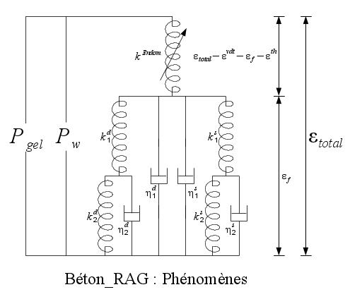
In order to model the difference in behavior, module VEP is split into two parts, a « spherical » part and a « deviatory » part. The spherical part (noted VEPs on the Figure 2.5.1-a) reflects the evolution of the structure of the CSH under hydrostatic stress linked to the departure of water as well as to the viscoplastic compression by generally isotropic « random » slides. The deviatory part reflects the sliding of the sheets subjected to shear stress. The pressure \({P}^{w}\) present on the Figure 2.5.1-a corresponds to the water pressure. It causes shrinkage if it is negative and swelling if it is positive.

\({P}_{w}\): intra porous water pressure
\({\mathrm{VEP}}^{s}\): spherical part of module VEP
\({\mathrm{VEP}}^{d}\): deviatory part of module VEP
Figure 2.5.1-a: Breakdown into spherical and deviatory parts of module VEP.
Given the heterogeneous nature of the porous distribution, we propose to model the phenomenon of creep as a hydromechanical consolidation problem in the following way: when a load is applied to the representative elementary volume (VER), interstitial overpressures appear in the water network, the first overpressures to disappear are those present in the water of the connected macroporosity, the load initially taken up by these overpressures is transferred to the skeleton solid (figure). This part therefore falls under classical hydromechanics. The solid skeleton itself consists, if observed on a finer scale, of a connected microporosity and a solid skeleton which will in turn be overloaded when the excess pressures present in its microporosity are evacuated to the macroporosity. Creep then appears as a succession of consolidation at increasingly finer scales, thus making use of less and less free water transfers. This interpretation of the creep phenomenon reveals a « fractal » nature of the consolidation mechanism, since the transfer of stresses to the solid skeleton takes place in an analogous manner at increasingly fine scales (figure), this hypothesis is also put forward by Acker [Acker, 2003]. At the finest scale, an irreversible nature of creep may be present; interfoliar water molecules are driven out irreversibly by the compression of hydrates.

Figure 2.5.1-b: Viscoelastic mechanisms associated with macroporosity
2.5.1.1. Spherical creep#

Figure 2.5.1.1-a: « Fractal » decomposition of spherical viscoelastic mechanisms
It is proposed to model these spherical creep mechanisms by three levels (figure), each level representing its own behavior.
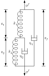
Figure 2.5.1.1-b: Spherical visco-elasto-plastic decomposition modeling spherical creep VEP
Level 0: This level is associated with macroporosity subjected to capillary pressure (\({P}_{w}\mathrm{=}{P}_{c}<0\)) if the medium is unsaturated, or to pore pressure (\({P}_{w}>0\)) if the model is used in a classical hydromechanical approach. So \({\sigma }_{0}^{s}\) is the effective stress on the solid skeleton. This level involves a purely elastic component of concrete. It can therefore be schematized and equated in the following way:
Level 1: This level corresponds to a part of the microporosity that is weakly connected to the open macroporosity and is subject to reversible water movements. The associated viscoelasticity is modelled by a Kelvin solid (figure):
: label: eq-4
{sigma} _ {1} ^ {s}mathrm {=} {k} _ {1} {varepsilon} _ {1} ^ {s} + {eta} _ {1} _ {1} {1} {1} {1} _ {1} ^ {s} {1} _ {1} ^ {s}
Level 2:
: label: eq-5
{sigma} _ {2} ^ {s}mathrm {=} {k} _ {2} {varepsilon} _ {2} ^ {s} + {eta} _ {2} _ {2} {2} {2} _ {2} ^ {s} {2} _ {2} ^ {s}
Level 2 corresponds here to the interfolliar nanoporosity of CSH. This level ensures the irreversible nature of the viscous deformations of CSH. In this last expression, \({k}_{2}\) is a kinematic work hardening module and \({\varepsilon }_{2}^{s}\) is an irreversible deformation. The rheological diagram makes it possible to establish the following system of equations:
2.5.1.2. Deviatoric creep#
In accordance with the observations of Acker et al. [Acker et al., 2003], Acker [Acker, 2001], Acker [], Bernard et al. [Bernard et al., 2003], the viscoelastic aspect of deviatoric behavior is attributed to the interfolliar shear of the CSH sheets. This shear occurs at two scales:
A viscoelastic nanoscopic scale corresponding to water weakly bound to the sheets,
A microscopic scale corresponding to free water weakly adsorbed between the sheets and subject to desiccation.
Finally, the part of the cement paste made up of better crystallized hydrates (portlandite and hydrated calcium aluminate) has an almost elastic behavior.
Deviatory viscosity therefore maintains a multi-scale nature, it is then proposed to represent it in a manner similar to the spherical branch, which also simplifies the implementation of the model (rheological equations similar to those of the deviatory branch).
The system managing the deformations of the deviatory rheological model is written as:
It can be specified at this stage of the modeling that the systems of rheological equations admit an analytical solution for a loading in linear total deformation as a function of time. We will take advantage of this solution in digital implementation.
2.5.2. Module dedicated to modeling the anisotropic swelling of RAG (VDt)#
The module in VDt (figure) models an increase in anelastic deformation when concrete is subjected to a tensile stress induced by RAG leading to damage.
We know that in the presence of RAG, the following deformation-damage relationship must be respected (figure):
In this equation, \({\mathrm{\epsilon }}_{0}\) is a parameter identified on a large number of tests and various types of concrete [Sellier, 1999]. Usually, its value is close to 0.35%.
\({d}_{i}^{\mathit{R0}}\) is a main value for the damage tensor due to tensile stresses induced by RAG. Here, it will be evaluated in the following way:
: label: EQ-None
{d} _ {i} ^ {R0} =mathit {min}left{{d} _ {i} ^ {t}; 1-text {exp}left (-frac {1} {1} {{1} {{m} {m}} {{m}} ^ {t}}} {left (frac {{b}} _ {g}. {P} _ {g}} {{mathrm {sigma}}} ^ {text {u t}}}right)} ^ {{m} ^ {t}}right}right)right}
In this expression, \({d}_{i}^{t}\) is a main value for the tensile damage tensor. \({m}^{t}\) and \({\mathrm{\sigma }}^{\text{u t}}\) are parameters of the law of evolution of damage. We will come back to the choice of damage variables and their law of evolution in the next chapter.
2.5.3. Assessment relating to the partitioning of deformations#
The proposed modeling for creep has been tested on multiaxial tests. Comparing simulations with experimental results shows the ability of the creep model to reproduce the characteristics of the long-term behavior of concrete. The next modeling step consists in setting up a damage model capable of representing the behavior of cracked concrete. This model will then be coupled with the natural creep model and the swelling model by the RAG described so far.
2.6. Damage model#
After giving the main principles of the model, we will first recall the thermodynamic concepts on which we must base our formulation. In a second step, we propose the free energy potentials and the complementary laws defining the model. This presentation makes it possible to verify the dissipation conditions imposed by the thermodynamics of the irreversible processes necessary for the convergence of calculations.
2.6.1. Principle of modeling#
The alkali-aggregate reaction causes swelling of the structure. These swellings can be very different depending on the loads of the damaged structures. Expansion that is considered isotropic when swelling is not prevented becomes a strongly anisotropic expansion as soon as concrete is subjected to a state of deviatoric stress [Multon, 2003; 2006]. Micro-cracking generated by intra-porous pressure is then prevented in the loading direction and swelling appears systematically associated with the directions where the compression stresses are the lowest. This phenomenon is particularly visible in beams where the cracks are oriented parallel to the reinforcements. A macro-cracking mechanism, due to the opening of cracks in the direction where the material is most damaged, amplifies this anisotropy. The micro and macro-cracks generated lead to a fall in the elastic modulus of concrete; this fall is usually modelled by damage theory. Below we present the principles of the damage model that we will apply to the stresses from the rheological diagram presented in the previous chapter.
In order to simulate the behavior of concrete degraded by the alkali-aggregate reaction, an anisotropic damage model, based on a realistic cracking criterion, must be used. This damage model must be formulated within the framework of thermodynamics [Lemaitre, 2001]. The thermodynamic framework makes it possible to avoid possible formulation inconsistencies that would lead to problems of physical representation and numerical convergence. To this end, a thermodynamic free energy potential from which the laws of material behavior derive must be proposed. In the case where mechanical dissipation can be decoupled from other dissipations (thermal, water or chemical), the dissipation condition is given by the Clausius-Duhem equation (equation). This relationship expresses the fact that the power of the « external forces » is at each moment greater than the recoverable power stored by the material; part of the power of the « external forces » being dissipated mechanically by decohesion, friction, etc. The Clausius-Duhem equation for an isothermal mechanical transformation is classically written:
In this expression, \(\sigma\) is the stress tensor, \(\varepsilon\) is the total strain tensor, is the total strain tensor, and \(\rho \psi\) is the volume free energy potential. The latter is chosen in such a way that the dissipation is zero in the case of perfectly elastic loading.
This restriction implies that the constraints \(\sigma\) derive from the free energy potential through the elastic deformations \({\epsilon }^{e}\), i.e.:
With the usual assumption of partitioning the total deformation:
Where \({\varepsilon }^{\text{an}}\) is anelastic deformation. Two internal variables, linked by this partition equation, are thus defined: anelastic deformation \({\varepsilon }^{\text{an}}\) and thermoelastic deformation \({\varepsilon }^{\text{e}}\). In our model, \({\varepsilon }^{\text{e}}\) is the deformation at level 0 of the rheological diagram; \({\varepsilon }^{\text{an}}\) contains the deformations \({\epsilon }_{\mathit{vdt}}\) and \({\epsilon }_{\mathit{vep}}\) shown in the figure as well as the thermal deformation if applicable.
The micro and macro cracks generated by the stresses lead to a fall in the elastic modulus of concrete; this fall is usually modelled by the theory of damage. Below are the principles of a damage model
The proposed model is based on a tensor representation of damage. This representation is formulated in such a way that the one-sided aspect of behavior can be dealt with simply and independently in each of the three main directions of effective constraints.
The effective stress tensor is estimated from the principle of equivalence in elastic deformation, at level 0 of the rheological diagram (figure):
With \({R}^{0}\) the fourth-order elasticity tensor of healthy concrete, calculated from the Young’s modulus and the Poisson’s ratio of uncracked concrete.
The apparent stresses are linked to the effective stresses by the damage tensor \(D\):
In this expression, (\(I\mathrm{-}D\)) an integrity tensor, also of the fourth order, consisting on the one hand of the identity matrix (\(I\)) and on the other hand of the damage tensor.
By treating the phenomenon of cracking using the fourth-order damage tensor \(D\), the free energy potential takes the following general form:
In index notation this last relationship is written:
Thus, the preceding equations lead to writing the Clausius-Duhem relationship in the following form:
Where \({V}^{\mathrm{an}}\) are the internal variables associated with anelastic deformations. Or again with the index notation:
This last relationship makes it possible to define the dissipation by anelastic deformation \({\phi }^{\text{an}}\) as well as the dissipation by mechanical damage \({\phi }^{D}\). It also makes it possible to define thermodynamic forces \({Y}_{\text{ijkl}}\), called energy restoration rates.
A simple way to ensure the positive nature of the dissipation regardless of the state of the material and of the charge is to postulate the decoupling of the dispersions by anelastic deformations and by damage, it is then necessary to verify separately \({\phi }^{\text{an}}\mathrm{\ge }0\) and \({\phi }^{D}\mathrm{\ge }0\) or again:
In viscoelasticity, the condition of dissipation by anelastic deformation leads to the choice of positive coefficients for viscosity laws.
In plasticity, we postulate the existence of a pseudodissipation potential (\({\phi }^{\text{*}\text{an}}\)). The latter being a positive convex function in the stress space and zero at the origin, so that the positivity of the dissipation is automatically verified. The flow law of anelastic deformations can be written in the form:
Where \(\dot{\lambda }\) is a positive scalar called a plastic multiplier. The latter is calculated so that the increase in anelastic deformation leads to a relaxation of the stresses, this making it possible to verify the plasticity criterion, which is also expressed in the stress space.
It remains to verify the positive condition of dissipation by damage. To do this, we can draw inspiration from the formalism briefly described above for plasticity. That is to say to give yourself a pseudodissipation potential that is convex and zero at the origin in the space of the energy restoration rates from which the increments of the components of the damage tensor derive. We then have the following law of evolution of damage:
: label: eq-20
{dot {D}} _ {text {ijkl}}}mathrm {=}mathrm {-}dot {lambda}frac {mathrm {partial} {partial} {phi} {phi}} ^ {text {ijkl}} ^ {text {ijkl}} ^ {text {ijkl}} ^ {text {*} D}} ^ {text {*} D}} ^ {text {*} D}}}
The « damage multiplier » \(\dot{\lambda }\) should be calculated in order to verify the damage criterion. The construction of the pseudopotential being arduous; the use of a more rational means, making it possible to ensure a form of the damage tensor consistent with the physical phenomena at the origin of the damage, is regularly used. To do this, the homogenization theory is used. The damage tensor \(D\) is estimated from the law of behavior of healthy material (\({R}^{0}\)) and from that of a representative elementary volume (VER) of cracked material (\({R}^{D}\)), it then comes from:
The representativeness of the law of behavior, of the damaged equivalent material will depend on the quality of the homogenization of VER. The unilateral nature of the behavior of concrete is induced by the restoration of stiffness associated with the re-closure of cracks. In the case of cyclic uniaxial loading with a change in the sign of the stress, it is possible experimentally to observe the creation of tensile cracks perpendicular to the loading axis and of compression cracks parallel to the loading axis. Tensile and compressive stiffness losses are therefore attributed to at least two orthogonal crack networks. When the stress changes from traction to compression, the tensile cracks are closed and the compression cracks are activated. When the stress changes from compression to tension, the tensile cracks open and are activated in turn.
To « physically » model the unilateral behavior of concrete, it is convenient to reason from a tensor description of the crack network. Tensile or compressive stiffness losses can thus be treated in each direction of space according to the sign of the stresses and the orientation of the cracks: if a main stress is positive, the most active cracks will be those whose orientation is generally perpendicular to the stress, whereas if the main stress is negative, the most active cracks will be parallel to the stress.
2.6.1.1. Anisotropic tensile damage#
The various reasons briefly stated above lead us to propose a damage model based on a representation of tensile cracking by a second-order tensor estimated from the effective tensile stress tensor \({\tilde{\sigma }}^{t}\) and not on extensions. These are the effective stresses in the sense of damage; they should not be confused with the effective stresses in the sense of the mechanics of porous media which affect the entire solid skeleton whereas the effective stresses in the sense of damage only affect the undamaged part of the solid skeleton.
The tensor of the effective tensile stresses is obtained from the main effective stresses, themselves resulting from the application of the principle of deformation equivalence to the rheological model used for the solid skeleton:
Where \({\overrightarrow{e}}^{i}\) is the eigenvector associated with \(\mathrm{\langle }{\tilde{\sigma }}_{i}\mathrm{\rangle }\) which is the positive part of the effective principal constraint \({\tilde{\sigma }}_{i}\).
Using the principle of deformation equivalence stated by Lemaître, the effective tensile stresses make it possible to define the tensor of the associated elastic deformations \({\varepsilon }^{\text{et}}\):
The cracking criterion used for tensile damage is that of Rankine, the threshold stress tensor is noted \({\sigma }^{R}\), the criterion translated in each main direction \({\overrightarrow{e}}^{i}\) of the effective stress tensor the failure to exceed the normal component of the threshold stress:
Updating the threshold stress tensor is in accordance with the consistency condition, which is simply written:
where \({\sigma }_{\text{ii}}^{R}\) are the terms of the diagonal of the \({\sigma }^{R}\) tensor expressed in the main base of effective constraints.
Assuming that the « equivalent » cracks, and therefore the damages, have the same main directions as the threshold stresses, we can define the damage tensor in the base of the main stresses of \({\sigma }^{R}\):
Damage \({d}^{t}\) represents a set of three orthogonal networks of plane cracks coexisting within the same representative elementary volume. The terms \({\overrightarrow{v}}^{i}\) are the eigenvectors of \({\sigma }^{R}\) and \({d}_{i}^{t}\) the eigenvalues of the damage tensor estimated from the eigenvalues \({\sigma }_{i}^{R}\) of \({\sigma }^{R}\), and the following law of evolution inspired by the Weibull law [Sellier, 1995].
Equation 2.6.1.1-1: Laws of evolution of damage
\({d}_{i}^{t}\mathrm{=}1\mathrm{-}\text{exp}(\underset{{\beta }_{i}}{\underset{\underbrace{}}{\mathrm{-}\frac{1}{{m}^{t}}{(\frac{{\sigma }_{i}^{R}}{{\sigma }^{\text{ut}}})}^{{m}^{t}}}})\)
In this expression \({m}^{t}\) is a parameter that is all the greater the more fragile the material is, \({\sigma }^{\mathit{ut}}\) is also a « material » parameter, it is similar to cohesion, in practice \({m}^{t}\) can be identified from the experimental damage measured from the peak of the law of behavior, \({\sigma }^{\mathit{ut}}\) is directly linked to the resistance. We will give the relationships between model parameters and measurable quantities in the following paragraphs. By introducing the crack index defined by:
: label: eq-27
{beta} _ {i}mathrm {=}frac {=}frac {1} {1} {{m}} {{m}} {{sigma} _ {i} ^ {R}}} {{sigma}}} {{sigma}}} {{sigma}}} {{sigma}}} {{sigma}}} {{sigma}}} {{sigma}}} {{sigma}}} {{sigma}}} {{sigma}}} {{sigma}}} {{sigma}}} {{sigma}}} {{sigma}
There comes the relationship between the damage and the crack index:
The latter relationship will be practical for the construction of free energy potential. The internal variables introduced at this level will also make it possible to memorize the state of cracking. In this context, it is also necessary to note that damage is an increasing and continuous function of the crack index, which is itself an increasing function of the threshold stress. Since the latter can only increase, the main values of the damage tensor can only increase.
With regard to normal deformation-stress relationships, the transition from the damage tensor to the law of behavior of the damaged material must reflect, on the one hand, a decrease in the Young’s modulus in the direction normal to the crack and, on the other hand, an attenuation of the Poisson effect between the direction orthogonal to the plane of the crack and the directions contained in its plane. To comply with these conditions, we propose to use the following law of behavior:
Again, depending on the signs of cracking:
: label: eq-30
{mathrm {epsilon}} _ {mathit {ii}}} ^ {e}} =frac {{mathrm {sigma}} _ {mathit {ii}} ^ {t}}} {{t}}} {{E}}} {{E}} ^ {0}}} {e}} {e}} ^ {mathrm {beta}} _ {i}}} -frac {{mathrm {mathrm {mathrm {nu}} ^ {0}} {{E} ^ {0}}} ({mathrm {sigma}} _ {mathit {jj}} ^ {t} + {mathrm {sigma}}} + {mathrm {sigma}}} + {mathrm {sigma}}} + {mathrm {sigma}}} _ {mathit {kk}} ^ {t})
In this expression \({E}^{0}\) is the Young’s modulus of the healthy material and \({\nu }^{0}\) is its Poisson’s ratio. The relationship is written into the main damage database. It should be noted that this law is expressed here as a function of apparent constraints and not of effective constraints. It is this particular writing that makes it possible to simply benefit from an attenuation of the Poisson effect as a function of the cracking in the \(j\) and \(k\) directions as well as of the symmetry of the flexibility tensor of the law of behavior. The slip-shear stress relationships are also written in the main damage base, the proposed relationship is as follows:
: label: eq-31
{mathrm {epsilon}} _ {mathit {ij}}} ^ {j}}} ^ {e} =frac {{mathrm {sigma}} _ {j}} ^ {t}} {2 {mathit {i}} ^ {t}}} {t}} {2 {mathrm {ij}}} {t}} {2 {mathrm {ij}}} {2 {mathrm {ij}}} {2 {mathrm {ij}}} {2 {mathrm {ij}}} {2 {mathrm {ij}}} {2 {mathrm {ij}}} {2 {mathrm {ij}}} {2 {mathrm {mu}}} {^ {t})}
Which can also be expressed in terms of cracking indices:
: label: eq-32
{mathrm {epsilon}} _ {mathit {ij}}} ^ {j}} ^ {e} =frac {{mathrm {sigma}} _ {mathit {ij}}} ^ {t}}} {t}} {2 {mathrm {t}}} {2 {mathrm {t}}}} {2 {mathrm {mu}}} {2 {mathrm {mu}}}} ^ {0}} {e}} ^ {mathrm {beta}}} _ {i}}} {i}} {i}} {i}} {2 {mathrm {mu}}} {2 {mathrm {mu}}} {mu}}} m {beta}} _ {j}}
The slip-shear stress relationship involves damage in the two main directions of cracking under shear stress; the combination of damages is of the weakest link type. In addition to the interaction between damages that this writing provides, it can be attributed a statistical meaning to it by considering that the damages are assimilated to the probabilities of encountering surface discontinuities on the facets [Sellier, 1995]. In this hypothesis, the weakest link theory indicates that the probability for a shear stress to transit on two orthogonal facets is equal to the probability of having two orthogonal surfaces that are not broken simultaneously. By neglecting the statistical dependencies between the two crack planes, this probability is equal to the product of the probabilities of having a continuity of the material on each of these two facets; the denominator of equation () is deduced therefrom. Finally, the last reason why we adopted this form for the damage of the shear coefficient is that the resulting law of behavior has the expected response to the rotation test of the main directions (known as the Willam test [Willam et al., 1987]).
To express the free energy potential as a function of elastic deformations, it is necessary to ensure the inversibility of the stress-strain relationships proposed previously. To do this, let us express the apparent normal stresses as a function of the elastic deformations:
\({\mathrm{\sigma }}_{\mathit{ii}}^{t}=\frac{{E}^{0}}{{D}^{n}}\left[\left({e}^{{\mathrm{\beta }}_{j}+{\mathrm{\beta }}_{k}}-{\mathrm{\nu }}^{{0}^{2}}\right){\mathrm{\epsilon }}_{\mathit{ii}}^{\mathit{et}}+{\mathrm{\nu }}^{0}{\mathrm{\epsilon }}_{\mathit{jj}}^{\mathit{et}}\left(\mathrm{\nu }+{e}^{{\mathrm{\beta }}_{k}}\right)+{\mathrm{\nu }}^{0}{\mathrm{\epsilon }}_{\mathit{kk}}^{\mathit{et}}\left(\mathrm{\nu }+{e}^{{\mathrm{\beta }}_{j}}\right)\right]\) with \({D}^{n}={e}^{{\mathrm{\beta }}_{i}+{\mathrm{\beta }}_{j}+{\mathrm{\beta }}_{k}}-{\mathrm{\nu }}^{{0}^{2}}\left({e}^{{\mathrm{\beta }}_{i}}+{e}^{{\mathrm{\beta }}_{j}}+{e}^{{\mathrm{\beta }}_{k}}\right)-2{\mathrm{\nu }}^{{0}^{3}}\) |
We show that \({D}^{n}\) is always positive if the following two conditions are met:
The condition on the Poisson’s ratio is verified, the same is true for the condition on \({\beta }_{i}\), taking into account the law of evolution of damages proposed previously. The inversibility of the normal deformation-normal stress relationship is therefore ensured regardless of the level of damage.
As far as the relationships between shear rates and shear stresses are concerned, the reversal is immediate and it comes from:
As the denominator of this expression is included in the interval \(\mathrm{[}\mathrm{1,}+\mathrm{\infty }\mathrm{[}\), inversibility is also ensured.
By integrating the stress-strain relationships with respect to the elastic deformations associated with the effective tensile stresses, the elastic free energy potential associated with the effective tensile stresses is obtained. This potential, noted \(\rho {\Psi }^{t}\) later, is expressed here in the main damage database:
And \({\text{ρψ}}^{t(s)}\) the one associated with elastic shear deformations:
The potential can also be expressed simply as a function of the apparent constraints \({\sigma }^{t}\) associated with the effective tensile stresses. In terms of the potential associated with extensions:
The \({E}_{i}\mathrm{=}{E}^{0}(1\mathrm{-}{d}_{i}^{t})\) being the Young modules of the damaged material. And for the potential associated with shears:
Since the cracks indices \({\beta }_{i}\) can be linked bijectively to the main tensile damages \({d}_{i}^{t}\), the Clausius-Duhem expression can be expressed as a function of the cracks indices. For greater clarity, we are temporarily ignoring the role of anelastic deformations here, assuming a damaging elastic transformation involving only effective tensile stresses:
In this expression, \({\epsilon }_{I}^{\text{et}}\) is a main value of the tensor of the deformations associated with the effective tensile stresses, \({\varphi }^{\text{Dt}(n)}\) is the dissipation associated with normal deformations and \({\varphi }^{\text{Dt}(s)}\) that associated with shear. \(R\) is the transition matrix from the main base of elastic deformations to the main base of damage, \(\dot{R}\) can be interpreted as a rotation rate of the damage tensor if the main directions of deformation do not rotate. Taking into account the shape of the free energy potential associated with shears then makes it possible to calculate the dissipation due to the damage associated with shears. It comes:
This expression is always positive since \({\dot{\mathrm{\beta }}}_{i}\) is positive, so the positivity of the dissipation associated with shears is verified.
With regard to the dissipation associated with normal deformations, we can notice that using the stress expressions for \({\psi }^{t(n)}\) and \({\epsilon }^{\text{et}}\) in the Clausius-Duhem equation, it comes:
Which means \({\dot{E}}_{i}\mathrm{\le }0\). Now that \({\dot{E}}_{i}\mathrm{=}\mathrm{-}{E}^{0}{\dot{d}}_{i}^{t}\) and \({\dot{d}}_{i}^{t}\) are positive, the second principle is also verified for damage associated with normal deformations.
In the case of non-radial loading, the Clausius-Duhem relationship contains terms due to changes in the main damages, which are always positive as we have just seen, as well as terms due to the rotations of the directions of damage. The latter reflect a convergence of the directions of orthotropy of the material and those of the loading. From an analytical point of view, this second transformation is analogous to a rotation of the main directions of deformation without damage. It therefore takes place without dissipation, so the following relationship must be respected at all times:
This involves:
Now, by construction, \(\mathrm{\sigma }=\mathrm{\rho }\frac{\partial {\mathrm{\Psi }}^{t}}{\partial {\mathrm{\epsilon }}^{\text{et}}}\), therefore, this condition is identically respected and the rotation of the damage directions does not lead to additional dissipation but induces a variation in the free energy potential compatible with the evolution of the load.
We have just presented the principles of an orthotropic damage model under effective stress, the latter enters the thermodynamic framework and also benefits from a direct numerical resolution method in accordance with (no sub-iterations at Gauss points). In fact, the calculation of the damage as a function of the effective stress is direct, as is the calculation of the apparent stress as a function of the effective stress and the damage.
2.6.1.2. Isotropic compression damage#
Under tensile stress, the criterion usually used is that of Rankine (main tensile stress), this criterion takes into account the propagation of cracks in \(I\) mode. In compression, the Mazars [Mazars, 1994] or Drücker-Prager criteria are commonly used; the Mazars criterion involves the notion of extending VER, the Drücker-Prager criterion takes into account the unfavorable effect of the constraint deviator. In practice, compression failure is induced by elastic heterogeneities leading to the appearance of local self-balanced stress fields, the positive part of which leads to the initiation and propagation of cracks (figure). Because of their origins, these induced positive stresses can only exist in directions orthogonal to the compression stresses that generate them. When these self-stresses reach the tensile strength, a crack starts and compression damage occurs. In ordinary concrete, this damage occurs gradually and it is possible to observe multiple vertical cracks distributed over a wide localized and inclined shear band (figure).

Figure 2.6.1.2-a: Crack facies as a function of the loading path [Torrenti1987]
The cracks parallel to the free edges are initiated in the vicinity of the aggregates by the induced self-stresses, they crack the concrete forming small « columns » which perish due to lateral instability as shown in the figure.

Figure 2.6.1.2-b: Appearance of « columns » in the vicinity of aggregates [Torrenti1987]
Thus, the propagation of compression cracks can be assimilated to a phenomenon of multiple instabilities in compression along a shear band. However, the phenomena of mechanical instability are very closely linked to the lateral maintenance conditions of the compressed element. Since instability always occurs in the weakest direction, this explains the cracks parallel to the unloaded edges in the figure.
In addition to the failure mode described above, it is important to remember how sensitive the compressive strength is to confinement as shown by the various biaxial and triaxial tests in the literature. Taking into account on the one hand the complexity of the compression failure mode and on the other hand the sensitivity to confinement, it is usual for modeling the damage of concrete in compression to adopt an isotropic macroscopic Drücker-Prager criterion if one reasons in terms of constraints, or a Mazars criterion if one reasons in terms of deformations. We have chosen here to adopt the Drücker-Prager criterion to be consistent with the effective stress formalism introduced when presenting the tensile damage model. The stresses causing compression damage are therefore assumed to be the negative effective stresses \({\tilde{\sigma }}^{c}\), the latter are defined in the main effective stress base by:
Where \(\tilde{\sigma }\) is the effective stress from the rheological model and \({\tilde{\sigma }}^{t}\) is the effective tensile stress defined by equation (). The equivalent Drücker-Prager stress is then written as:
Where \({I}_{1}\) and \({J}_{2}\) are the first two invariants of the effective compression stress tensor:
The flow is carried out by considering that the damage threshold stress stores the maximum value of the Drücker-Prager stress:
The damage then evolves nonlinearly as a function of the threshold stress:
: label: eq-50
{d} ^ {c}mathrm {=}} 1mathrm {-}text {exp} (mathrm {-}frac {1} {{m} ^ {c}}} {(frac {{sigma}}} {frac {sigma}}} {text {uc}}}} {{m} ^ {c}}} {(frac {sigma}}}} {frac {sigma}}} {text {uc}}}} {{m} ^ {c}}} {(frac {sigma}}}} {frac {sigma}}} {{m} ^ {c}}} {(frac {sigma}}})} {{m} ^ {c}}} {})
The free energy potential associated with effective compression stresses can be written very simply due to the hypothesis of isotropy of compression damage:
The dissipation associated with compression damage is written as:
: label: eq-52
{phi} ^ {text {dc}}mathrm {=}mathrm {=}mathrm {-}underset {{Y} ^ {c}} {underset {underbrace {}}} {rhofrac {frac {frac {frac} {mathrm {partial}}} {rhofrac {frac} {frac {mathrm {partial}}} {mathrm {partial}} {d}rhofrac {frac {frac} {frac {mathrm {partial}}} {mathrm {partial}} {d}rhofrac {frac {frac} {fracdot {d}} ^ {c}
Since the \({Y}^{c}\) energy recovery rate is negative and the damage is strictly increasing, the positivity of dissipation through compression damage is assured.
2.6.1.3. Coupling of tensile and compression damages#
The predominant isotropic nature of compression damage is linked to the « almost random and therefore statistically isotropic » complexity of the crack paths generated during the degradation process. It is obvious that the cracks created will affect the tensile behavior. A simple way to account for the decrease in elastic moduli in tension as a function of compression damage is to consider that isotropic compression damage also reduces the free tensile energy potential, which becomes:
The term \(\rho {\psi }^{t}\) being positive, the positivity of dissipation due to compression damage remains assured:
And since the term \((1\mathrm{-}{d}^{c})\) is also positive, the dissipation due to traction damage remains positive.
Free energy potential associated with macroscopic elastic deformations
The partition of the deformations according to the sign of the effective stresses being made equations () and (), the free energy potential is the sum of the free energies associated with the effective tensile stresses on the one hand and with the effective compressive stresses on the other hand:
Free energy potential associated with an expansive internal chemical reaction
If the model integrates a pressure (\({P}_{g}\)) created by the expansive chemical reaction in progress \(A\), the free energy potential, at a given temperature and at a given time, becomes a function of \(A\):
In this expression \({V}^{\mathit{an}}\) represents the internal variables associated with anelastic phenomena. The Clausius-Duhem inequality therefore becomes:
In this expression, the term \({P}_{g}(\dot{A}{V}^{g})\) is the mechanical power provided to the solid skeleton by the chemical reaction. If we consider a physical transformation of VER without damage or anelastic deformation, and therefore without mechanical dissipation, this energy must be found entirely in the free energy potential, which can be written:
On the other hand, physical considerations lead us to express the gel pressure as a function of the volume fraction of excess material compared to the volume of voids connected to the reactive site on the one hand and total deformations on the other hand, equation ().
Respecting the two previous relationships leads to the following form being proposed for the portion of the potential due to the freeze:
This form of potential is similar to that proposed by Ulm et al. [Ulm et al., 2002]. The derivative of this potential with respect to elastic deformations gives the part of the macroscopic stress induced by the internal gel pressure in the solid skeleton:
2.6.1.4. Free energy potentials associated with water pressures#
In a saturated medium, intra porous pressures act on the solid skeleton by deforming the walls of the porous network; the Clausius-Duhem equation is written, in the absence of damage and anelastic phenomena:
In this expression \({\varphi }^{w}\mathrm{=}\frac{{m}^{w}}{{\rho }^{\mathit{w0}}}\) is the standardized water mass input, \({m}^{w}\) being the mass input and \({\rho }^{\mathit{w0}}\) the density of water defined at the reference pressure \({P}_{\mathit{w0}}\). Moreover, physical considerations lead to the expression of water pressure in the form [Coussy, 2002]:
: label: eq-62
{P} _ {w}mathrm {-} {P} {P} _ {mathit {w0}}mathrm {=} {M} ^ {w} ({varphi} ^ {w}mathrm {-} {w}mathrm {-} {w}}mathrm {-} {b}} ^ {w}text {tr} (varepsilon))
An acceptable form for the free energy potential associated with these equations is then:
The derivative of this potential with respect to elastic deformations gives the part of the macroscopic stress induced by water pressure:
If the reference state is defined for the saturated material at atmospheric pressure \(({P}_{\mathit{w0}}\mathrm{=}0)\), then the previous expression is only valid if the fluid mass input is positive. Otherwise, the concrete is de-saturated and the water pressure is no longer managed by the relative compressibilities of the various phases but by capillary phenomena. The average water pressure \({P}_{w}\) is therefore a function of the capillary pressure and the degree of saturation \({S}^{w}\). In addition to the variation in pressure in water induced by capillary phenomena, it is also necessary to consider the action of the interfaces of the fluid with the gaseous medium and the solid. In fact, these interfaces are subject to capillary tension phenomena which also act directly on the solid skeleton. In the case where the pressure of the intra porous gas is in equilibrium with the atmospheric pressure [Coussy, 2002], the part of the macroscopic stress induced by these two phenomena can be put into the following general form:
Where \({f}^{w}\) is a function taking into account on the one hand the decrease in the volume of water and on the other hand the increase in the number of solid sites subject to interface surface tension. In the present modeling, we are interested in structures located in a partially saturated zone, in this case we propose to use a linear \({f}^{w}\) function of the form \({k}^{w}\mathrm{\cdot }{S}^{w}\), the contribution of water effects in the macroscopic stress then has the following form:
Considering that the variation in porosity \(\varphi\) due to deformation remains small compared to \({\varphi }^{w}\), it can be assumed that for the unsaturated medium \(\varphi \mathrm{\approx }{\varphi }^{0}\). If, on the other hand, it is accepted that the capillary pressure curve \({P}^{c}({S}^{w})\) is virtually insensitive to the state of deformation of the solid skeleton, then:
If the capillary pressure curve has a « Van Genuchten » equation, then \({\pi }^{w}\) takes the following form:
Where \(a\) and \(b\) are two calibration constants.
The free energy potential can then be in the form of:
The thermodynamic force associated with the variation in the mass of water is obtained by deriving this potential with respect to \({\varphi }^{w}\).
2.6.1.5. Dissipation due to anelastic deformations#
The Clausius-Duhem equation reveals anelastic deformations \({\varepsilon }^{\text{an}}\) in the term \(\sigma \mathrm{:}{\dot{\varepsilon }}^{\text{an}}\). This is the power of the external forces of the anelastic deformation field, the evolution of these deformations induces an evolution of the associated internal variables \({V}^{\mathit{an}}\) possibly causing a variation in the free energy potential:
The latter term represents the elastic energy that is blocked in the solid skeleton by anelastic deformation. In our model, anelastic deformations have a viscoelastic or viscoplastic origin and can be directly used as internal variables, i.e. \({V}^{\text{an}}\mathrm{=}{\varepsilon }^{\text{an}}\).
Thus, in the particular case of a purely anelastic transformation, the dissipation comes down to:
: label: eq-71
{phi} ^ {text {an}}mathrm {-}mathrm {=}sigmamathrm {:} {dot {varepsilon}} ^ {text {an}}mathrm {-}mathrm {-} -}rhofrac {frac {frac {frac {frac {frac {frac {frac {text}psi} {mathrm {partial} {partial} {partial} {partial} {partial} {text} {varepsilon}}mathrm {-} -}mathrm {- -}rhofrac {frac {frac {frac {frac {year}} {dot {varepsilon}}} ^ {text {an}}mathrm {ge} 0
In the model proposed here, we adopted the principle of partitioning the total deformation into elastic parts and anelastic parts, which makes it possible to express the elastic deformations as a function of the anelastic deformations and to conclude that the thermodynamic force associated with the anelastic deformation is the stress:
So the second principle is true if \(\sigma \mathrm{:}{\dot{\varepsilon }}^{\text{an}}\mathrm{\ge }0\). In the model studied here, the anelastic deformation associated with long-term creep or expansive chemical reaction is proportional to the stress, which can be written in the abbreviated form \({\dot{\varepsilon }}^{\text{an}}\mathrm{=}k\sigma\), where \(k\) is a positive coefficient dependent on internal variables for each component of the strain tensor. Thus anelastic dissipation due to long-term deformations is a viscous dissipation of the form \(k{\sigma }^{2}\mathrm{\ge }0\). Regarding the deformation of RAG, we only allow its evolution if the dissipation calculated numerically over the time step is actually positive.
2.6.1.6. Total free energy potential and state laws#
The free energy potential of the solid skeleton is obtained by summing the energy contributions of the various phenomena studied previously:
State laws are obtained by deriving the total potential:
If one expresses stresses in the main basis of tensile damage, it comes for the diagonal terms of the stress tensor:
and for terms that are off the diagonal:
With \({D}^{n}\mathrm{=}{e}^{{\beta }_{i}+{\beta }_{j}+{\beta }_{k}}\mathrm{-}{\nu }^{{0}^{2}}({e}^{{\beta }_{i}}+{e}^{{\beta }_{j}}+{e}^{{\beta }_{k}}+2{\nu }^{0})\) and \({e}^{{\beta }_{i}}\mathrm{=}\frac{1}{1\mathrm{-}{d}_{i}^{t}}\)
Recall that the elastic deformations of traction \({\varepsilon }^{\text{et}}\) and compression \({\varepsilon }^{\text{ec}}\) result from two successive decompositions, the partition of the total deformation on the one hand:
and on the other hand of the partition depending on the sign of the effective stress in the sense of damage:
And the thermal deformation equation:
In equation (), \({\varepsilon }^{\text{th}}\) is the deformation due to thermal expansion defined classically by equation () where \({\alpha }^{\theta }\) is the thermal expansion coefficient, \(T\) the temperature and \({T}_{0}\) the reference temperature. Note that in equation (), a reference deformation \({\varepsilon }^{0}\) is also present, it is a non-zero reference deformation corresponding to a stress-free state. It can only be associated with a volume variation in the solid skeleton of chemical origin (chemical withdrawal due to hydration for example). In fact, deformations of water withdrawal or swelling by internal expansive products are manifestations of intra porous pressures appearing via elastic and anelastic deformations, they should therefore not be confused with this « chemical deformation imposed by reference » which is not accompanied by internal pressures and cannot therefore create damage through free deformation.
The elastic and anelastic deformations are obtained by solving the system of rheological equations presented in the previous chapter. If the resolution of the system of equations of the rheological model is direct (without nonlinearity requiring numerical sub-iterations at the Gauss point in the finite element implementation), then the resolution of the entire model is direct for the total deformation field data. Recall that this aspect of the model meets the objective of ease of implementation and reduction of calculation time that we initially set ourselves. The table below summarizes the variables.
Table 2.6.1.6-1: Thermodynamic variables.
State variables |
Related variables |
|
Observables |
Internals |
|
\(\mathrm{\epsilon }\) |
\(\mathrm{\sigma }\) |
|
T |
S |
|
\({\mathrm{\epsilon }}^{e}\) |
\(\mathrm{\sigma }\) |
|
\({\mathrm{\epsilon }}^{\mathit{an}}\) |
\(-\mathrm{\sigma }\) |
|
\({d}^{t}\) |
\({Y}^{t}\) |
|
\({d}^{c}\) |
\({Y}^{c}\) |
|
\(A{V}_{g}\) |
\({P}_{g}\) |
|
\({\mathrm{\varphi }}^{w}\) |
\({P}_{w}\) |
|
2.6.2. Coupling the damage model and the rheological model#
Since the rheological model and the damage model have been described individually in the preceding paragraphs, they must now be linked. As mentioned in the previous paragraph, the effective stresses and deformations referred to in the damage model chapter are derived from the rheological diagram. The coupling between viscoelastic phenomena and damage therefore consists in defining on the rheological diagram the effective stresses and the deformations to be used to calculate the damage. Currently, the effective stresses used in the damage model come directly from the rheological model for which the integration of the equations () and () is carried out with the viscoelastic characteristics of the healthy material. The coupling between damage and rheology is therefore immediate. In fact, if the damage increases during a creep test, then the effective stresses will increase in the rheological model, leading to an increase in the creep speed.