1. Theoretical formulation

1.1. Behavioral relationship of Hujeux

The model described here is the so-called Hujeux model. The model was developed by École Centrale Paris (laboratory LMSSMat) in the 1980s in order to represent the rheology of soils for alternating loads, for example in earthquakes. This soil mechanical behavior relationship is a multi-mechanism model, characterized by two times four load surfaces with work hardening: three linked to deviatory mechanisms and one to a spherical consolidation mechanism, defined for monotonic paths and for cyclic paths. The deviatory mechanisms are defined on three fixed planes, which induces an orthotropy of soil behavior. Spherical mechanisms reproduce the strong non-linearity of geomaterials on a consolidation path.

Each of these planes, indexed by \(k\), is defined by the base vectors \(({{e}_{i}}_{k},{{e}_{j}}_{k})\), extracted from the orthonormal base \(({e}_{1},{e}_{2},{e}_{3})\) of the 3-dimensional space. We note the indices:

\({i}_{k}=1+\text{mod}(\text{k,}3)\) and \({j}_{k}=1+\text{mod}(\text{k+}\text{1,}3)\) eq 1.1 -1

Note:

In a 2D plane deformation situation, the plane \(\text{k=}3\) corresponds to the plane \(({\mathrm{e}}_{1},{\mathrm{e}}_{2})\) of the model.

The model has a nonlinear elasticity controlled by the Young’s modulus depending on the confinement pressure.

A three-dimensional limit criterion similar to that of Mohr-Coulomb is considered to take into account the influence of the effective mean stress on the stiffness of the ground and of the fracture characteristics. The concept of critical state is also integrated into this model to represent the coupling between deviatory stresses and volume variations and to formulate isotropic work hardening related to the granular medium. Kinematic work hardening is added to represent the cyclical behavior of soils and coupled with ground density work hardening.

The Hujeux model is expressed in effective constraints —defined as being the difference between total stresses and water pressure in the case of saturated soils— in the case of hydromechanical coupling: i.e. we do not take into account the hydrostatic pressure of the fluid that can circulate in the pores, this being calculated in models THM.

1.1.1. Definition of state variables and expression of free energy

1.1.1.1. State variables

The variables used to describe the condition of the material point are as follows:

• \(\varepsilon\): deformation tensor,

• \({\varepsilon }^{p}\): plastic deformation tensor; \({\mathrm{\varepsilon }}_{v}^{p}=\text{tr}{\mathrm{\varepsilon }}^{p}={\mathrm{\varepsilon }}^{p}\text{.}I\) is especially noted for volume plastic deformation, \(\mathrm{I}\) being the identity tensor,

• \({r}_{k}^{m}\): the « mobilization factors » of deviatory mechanisms in a monotonic path: it is a work hardening in the pressure-shear plane,

• \({r}_{k}^{c}\): the « mobilization factors » of cyclic deviatory mechanisms: it is a mixed isotropic and kinematic work hardening in the pressure-shear plane.

• \({r}_{4}^{m}\): the factor of mobilization of the consolidation mechanism in a monotonic path: it is a hardening of the spherical consolidation mechanism (scalar),

• \({r}_{4}^{c}\): the factor for mobilizing the consolidation mechanism in a cyclic path: it is a mixed isotropic and kinematic (scalar) work hardening,

accompanied by a number of discontinuous story variables, described below.

The various mechanisms of elastoplastic evolution involve work-hardening variables: the mobilization factors associated with each of the mechanisms and the plastic volume deformation \({\mathrm{\varepsilon }}_{v}^{p}=\text{tr}{\mathrm{\varepsilon }}^{p}\), common to all the mechanisms and coupling them. The latter modifies the load surfaces even if they are not active, due to the work hardening carried out on the other activated load surfaces: see [§ 1.1.2 and 1.1.3].

\(\sigma ` denotes the stress tensor (effective), the confinement pressure being: :math:`p(\mathrm{\sigma })=\frac{1}{3}\text{tr}(\mathrm{\sigma })\). By convention in*Code_Aster*, the compression case corresponds to negative stresses (and deformations). For each plastic mechanism in plane \(k\), we denote by:

\({\sigma }_{(k)}={P}_{(k)}\cdot \sigma \cdot {P}_{(k)}\) eq 1.1.1-1

the constraints in plane \(k\), where \({P}_{(k)}\) refers to the (symmetric) projection tensor on the base plane \(({e}_{{i}_{k}},{e}_{{j}_{k}})\), with normal \({e}_{k}\):

\({P}_{(k)}={e}_{{i}_{k}}\otimes {e}_{{j}_{k}}+{e}_{{j}_{k}}\otimes {e}_{{i}_{k}}\) eq 1.1.1-2

with \({i}_{k}=1+\text{mod}(k\mathrm{,3})\) and \({j}_{k}=1+\text{mod}(k+\mathrm{1,3})\), i.e.:

\({\sigma }_{(k)}={\sigma }_{{i}_{k}{i}_{k}}\text{.}{e}_{{i}_{k}}\otimes {e}_{{i}_{k}}+{\sigma }_{{j}_{k}{j}_{k}}\text{.}{e}_{{j}_{k}}\otimes {e}_{{j}_{k}}+{\sigma }_{{i}_{k}{j}_{k}}\text{.}{e}_{{i}_{k}}{\otimes }_{s}{e}_{{j}_{k}}\) eq 1.1.1-3

then the confinement pressure in plane \(k\):

\({p}_{k}(\sigma )=\frac{1}{2}\text{tr}({\sigma }_{(k)})\) eq 1.1.1-4

We also define the deviatory stress tensor \({S}_{(k)}\) in the \(k\) plane, using the 2nd order identity tensor in the plane: \({I}_{(k)}={\delta }_{{i}_{k}{j}_{k}}{e}_{{i}_{k}}\otimes {e}_{{j}_{k}}\):

\({S}_{(k)}(\mathrm{\sigma })={\mathrm{\sigma }}_{(k)}-{p}_{k}(\sigma )\text{.}{I}_{(k)}\) eq 1.1.1-5

We have \(\mathrm{tr}{S}_{(k)}=0\). Finally, we note the norm (von Mises) of the deviatory stress tensor \({S}_{(k)}\):

\({q}_{k}(\sigma )={∥{S}_{(k)}(\sigma )∥}_{\text{VM}}^{\text{2D}}=\sqrt{\frac{1}{2}{S}_{(k)\alpha \beta }\text{.}{S}_{(k)}^{\alpha \beta }}\) eq 1.1.1-6

Moreover, several variables that remember an irreversible history preserve during certain phases of evolution the values of the state variables at the beginning of these phases, and govern subsequent evolutions, recording the value of this variable at the beginning of the path where a cyclic mechanism is activated:

• \({p}_{H}\): memorizing discontinuous scalar variable, recording the value of the confinement pressure \(p(\mathrm{\sigma })\),

• \({\varepsilon }_{\mathrm{vH}}^{p}\): memorizing discontinuous scalar variable, recording the value of the volume plastic deformation,

• \({p}_{\text{kH}}\): discontinuous memory scalar variable, recording the value of the « confinement pressure of the \(k\) plane » \({p}_{k}\),

• \({S}_{(k)H}\): discontinuous memory tensor variable, recording the value of the deviators of the \({S}_{(k)H}(\mathrm{\sigma })\) constraints in each plane \(k\), whose expression is given in [éq1.1.1-5],

• \({S}_{(k)H}^{c}\): discontinuous memory tensor variable, recording the value of the deviators of the « modified » constraints \({S}_{(k)}^{c}(\mathrm{\sigma },{\mathrm{\varepsilon }}_{v}^{p}{\text{,r}}_{k}^{c})\) in each deviator plane \(k\), whose expression is given in [éq1.1.2-12].

Note:

The formulation by orthogonal plans of the Hujeux model does not allow axisymmetric states to be represented correctly; cf. [bib9] _*.*

1.1.1.2. free energy

We denote free energy by the sum of an elastic contribution and a work hardening contribution:

\(\begin{array}{}F(\varepsilon (\overrightarrow{u}),{\varepsilon }^{p},{r}_{k}^{K})={F}_{\text{él}}(\varepsilon (\overrightarrow{u}),{\varepsilon }^{p})+{H}_{\text{écr}}({\varepsilon }_{v}^{p},{r}_{k}^{K})\end{array}\) eq 1.1.1-7

for \(K=m,c\); \(\text{k=}\text{1,}\text{.}\text{.}\text{.}\text{,4}\). Thermodynamic dissipation is obtained by difference from the deformation power density, this in an isothermal process:

\(D=\sigma \text{.}\varepsilon (\dot{\overrightarrow{u}})-\dot{F}(\varepsilon (\overrightarrow{u}),{\varepsilon }^{p},{r}_{k}^{K})=\sigma \text{.}{\dot{\varepsilon }}^{p}-{\dot{H}}_{\text{écr}}({\varepsilon }_{v}^{p},{r}_{k}^{K})\) eq 1.1.1-8

Insofar as the thermal coupling is not resolved, it is not possible to differentiate the density of power dissipated from the rate of work hardening energy, corresponding to a term of blocked energy. However \(\sigma \cdot {\dot{\varepsilon }}^{p}\) is not necessarily a positive step, unlike \(D\). As will be seen below, the elastic part of Hujeux’s law is non-linear: it is not easy to extract the expression for the \({F}_{\text{él}}(\varepsilon (\overrightarrow{u}),{\varepsilon }^{p})\) potential.

As Hujeux’s law of behavior has a particular nonlinear elasticity, cf. [§ 1.1.1.3], one cannot give the integrated expression of free energy.

1.1.1.3. Hujeux’s nonlinear elastoplastic law

It is assumed that the Young’s modulus of the soil depends on the confinement pressure \(p(\sigma )\) by a power law, in the field of compressions \(p(\sigma )<0\). The Hujeux nonlinear elastoplastic behavior relationship is written as:

\(\sigma =\frac{\partial }{\partial \varepsilon }{F}_{\text{él}}(\varepsilon (\overrightarrow{u}),{\varepsilon }^{p})=C(p)\text{.}(\varepsilon (\overrightarrow{u})-{\varepsilon }^{p})\) eq 1.1.1-9

where elasticity tensor \(C(p)\) is isotropic.

In practice, the relationship [éq 1.1.1.9] cannot be expressed in analytical form, and the relationship between elastic volume deformation and confinement pressure is identified in incremental (hypoelastic) form:

\(\dot{p}=\frac{{K}_{0}}{1-n}\text{.}{∣\frac{p(\sigma )}{{P}_{\text{réf}}}∣}^{n}\text{.}\text{tr}(\dot{\varepsilon }-{\dot{\varepsilon }}^{p})\) eq 1.1.1-10

where two parameters are defined: \(n\in [\text{0,}1[\) and \({P}_{\text{réf}}\) (not zero), as well as the initial modules \({E}_{0}\) and \({\mathrm{\nu }}_{0}\) (or, according to soil mechanics practice, the initial positive shear and \({K}_{0}\) compressibility moduli measured at the reference confinement pressure \({P}_{\mathrm{réf}}\)), which define the initial elasticity tensor \({G}_{0}\) \({C}^{0}\). Case \(n=0\) corresponds to linear elasticity.

The components of the elasticity tensor of the nonlinear elastic law are therefore written as:

\({C}_{\text{ijkl}}(p){\text{=C}}_{\text{ijkl}}^{0}\text{.}{∣\frac{p(\mathrm{\sigma })}{{P}_{\text{réf}}}∣}^{n}{\text{=G}}_{0}\text{.}({\mathrm{\delta }}_{\text{ik}}{\mathrm{\delta }}_{\text{jl}}{\text{+\delta }}_{\text{jk}}{\mathrm{\delta }}_{\text{il}}+\frac{2{\mathrm{\nu }}_{0}}{1-2{\mathrm{\nu }}_{0}}{\mathrm{\delta }}_{\text{ij}}{\mathrm{\delta }}_{\text{kl}})\text{.}{∣\frac{p(\mathrm{\sigma })}{{P}_{\text{réf}}}∣}^{n}\) eq 1.1.1-11

The compressibility coefficient will be noted below:

\(K(p)={K}_{0}\text{.}{∣\frac{p(\mathrm{\sigma })}{{P}_{\text{réf}}}∣}^{n}\) eq 1.1.1-12

It can be seen that the elastic law is not differentiable if the confinement pressure is zero (and if \(n\ne 0\)). In practice, this law leads to greater soil stiffness the deeper you go down.

The criteria (or plastic load surfaces) involve the critical pressure function, which characterizes the resistance of the soil, depending on the index of voids in the material (density work hardening):

\({P}_{c}({\mathrm{\varepsilon }}_{v}^{p}){\text{=P}}_{\text{c0}}\text{.}{e}^{-{\text{\beta \varepsilon }}_{v}^{p}}\) eq 1.1.1-13

where two material parameters are involved: initial critical reference pressure \({P}_{\mathrm{c0}}\) (negative) and \(\beta\) the plastic compressibility of the material (positive). The critical pressure increases in absolute value when the material has undergone negative volume plastic deformation (compression).

1.1.2. Deviatory elastoplastic mechanisms

Three deviatory mechanisms are considered: one in each sliding plane \(k\) (normal \({e}_{k}\)); in addition, we identify a valid behavior during the local monotonic load paths, and another behavior, controlled by a story-memory variable, on the cyclic loading paths (from the moment of discharge from the state reached at the end of a monotonic path).

1.1.2.1. Deviatory criteria in monotonic loading

The deviatory mechanisms in plane \(({{e}_{i}}_{k},{{e}_{j}}_{k})\) for a monotonic journey are governed by the criterion:

\({f}_{k}^{m}(\sigma ,{\varepsilon }_{v}^{p}{\text{,r}}_{k}^{m})={q}_{k}(\sigma ){\text{+p}}_{k}(\sigma )\text{.}F({p}_{k}(\sigma ),{\varepsilon }_{v}^{p})\text{.}({r}_{k}^{m}{\text{+r}}_{\text{éla}}^{d})\le 0\) eq 1.1.2-1

with:

\({p}_{k}(\mathrm{\sigma })\) and \({q}_{k}(\mathrm{\sigma })\) defined in [eq 1.1.1 -5], [eq 1.1.1 -6] and [eq 7 -2];

and the function that characterizes soil resistance as a function of volume plastic deformation:

\(F({p}_{k}(\sigma ),{\varepsilon }_{v}^{p})=M\text{.}(1-{b}_{h}\text{ln}∣\frac{{p}_{k}(\sigma )}{{P}_{c}({\varepsilon }_{v}^{p})}∣)\) \(\Rightarrow \frac{\partial F}{\partial {p}_{k}}=-\frac{{b}_{h}M}{{p}_{k}};\frac{\partial F}{\partial {\varepsilon }_{v}^{p}}=-{b}_{h}\beta M\) eq 1.1.2-2

where three other material parameters are involved: \(M=\text{sin}{\varphi }_{\mathrm{pp}}\) (\({\varphi }_{\mathrm{pp}}\) is the angle of internal friction), the positive coefficient \({b}_{h}\) and the parameter \({r}_{\text{éla}}^{d}\in ]\text{0,1}[\) which characterizes the size of the threshold in the initial state); the critical pressure \({P}_{c}({\varepsilon }_{v}^{p})\) is defined by [eq 1.1.1 -13].

The criterion [eq 1.1.2 -1] is strongly inspired by the original Cam-Clay [bib8] _ model. However, the expression was modified by Hujeux [bib4] _, because this model underestimated deviatory deformations for over-consolidated clays. To correct this weakness, he modified the load surface by introducing a dependence on deviatory deformations without changing the Roscoe [bib7] _ expansion volume flow rule, cf. [§ 1.1.2 .2], cf. [§ .2]. Compared to Cam-Clay, the Hujeux model makes it possible to better model cycles.

[fig. 1.1 -a] visualizes the effect of the critical pressure \({P}_{c}({\varepsilon }_{v}^{p})\) and the mobilization factor \({r}_{k}^{m}\) on the threshold positioned in relation to the critical state line (angle \({\varphi }_{\mathrm{pp}}\)) and to the dilatance line (angle \(\mathrm{\psi }\), cf. [eq 1.1.2 .3]).

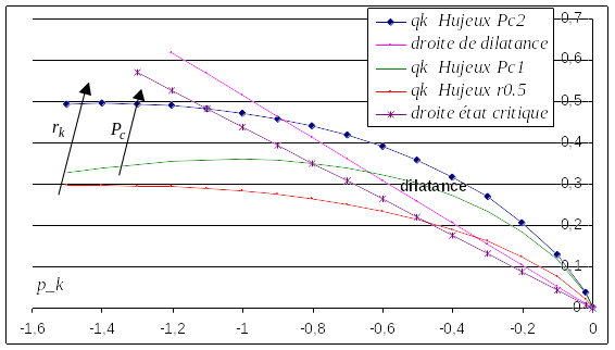
Figure 1.1 -a: Deviatory load surfaces (in the stress plane \({p}_{k}(\mathrm{\sigma }),{q}_{k}(\mathrm{\sigma })\) ) .

Note:

We can reformulate the monotonic criterion [eq 1.1.2 -1] by normalizing the equivalent stress \({q}_{k}(\sigma )\) by \({p}_{k}(\sigma )\text{.}F({p}_{k}(\sigma ),{\varepsilon }_{v}^{p})\) , in such a way that we can interpret the criterion geometrically by a circle with radius \({r}_{k}^{m}{\text{+r}}_{\text{éla}}^{d}\) :: :math:`{tilde{f}}_{k}^{m}(sigma ,{varepsilon }_{v}^{p},{r}_{k}^{m})={tilde{q}}_{k}(sigma ,{varepsilon }_{v}^{p})-({r}_{k}^{m}+{r}_{text{éla}}^{d})le 0`, cf. [:ref:`fig. 1.1-b <fig. 1.1-b>`] . *

The criterion [éq 1 *.1.2-1] requires the presence of an initial state of consolidation*:math:`{p}_{k}(sigma )ne 0`*in the material so that the threshold is not zero. *

Note:

Soil liquefaction is the situation that occurs when the effective consolidation pressure of the soil is close to zero. This state can occur after a cyclic loading, for example for loose sands, but also for monotonous loading, on loose sand in undrained conditions.

1.1.2.2. Flow and work hardening laws under monotonic loading for deviatory mechanisms

The first part of the plastic deformation velocities for the deviatory mechanism is divided into a purely deviatory part, respecting an associated flow law (normal flow), and a spherical, non-associated part, respecting the principles of Roscoe’s law of dilatance [bib7] _. It is a « non-generalized standard material. » The flow law is written as follows:

\({({\dot{\varepsilon }}^{p})}_{(k)}^{m}={\dot{\lambda }}_{k}^{m}\text{.}{\Psi }_{(k)}^{m}={\dot{\lambda }}_{k}^{m}\text{.}(\frac{{S}_{(k)}}{{\text{2q}}_{k}}-\frac{{\zeta }_{0}\text{.}\zeta ({r}_{k}^{m}{\text{+r}}_{\text{éla}}^{d})}{2}\text{.}(\text{sin}\psi +\frac{{q}_{k}}{{p}_{k}})\text{.}{I}_{(k)})\) eq 1.1.2-3

Tensor \({\Psi }_{(k)}^{m}\) refers to the flow direction. The expansion angle \(\psi ` and :math:`{\zeta }_{0}\) are material parameters. The \(\zeta (r)\) function makes it possible to control the effect of volume variation during a plastic flow on a diverting mechanism (flow which is then non-standard). Up to a certain level of shear, the variation in volume is zero; beyond that, it occurs. The expression for function \(\zeta (r)\) is:

\(\zeta (r)=\left\{\begin{array}{ccc}0& \text{si}r\le {r}_{\text{hys}}& \text{domaine}\text{pseudo}-\text{élastique}\\ {(\frac{r-{r}_{\text{hys}}}{{r}_{\text{mob}}-{r}_{\text{hys}}})}^{{x}_{m}}& \text{si}{r}_{\text{hys}}<r\le {r}_{\text{mob}}& \text{domaine}\text{hystérétique}\\ 1& \text{si}{\text{r>r}}_{\text{mob}}& \text{domaine}\text{plastique}\end{array}\right\}\) eq 1.1.2-4

where \({r}_{\text{hys}},{r}_{\text{mob}},{x}_{m}\) are new parameters for deviatory mechanisms.

We call characteristic state the situation corresponding to evolutions where \({\dot{\mathrm{\varepsilon }}}_{v}^{p}=0\) (zero evolution of contract). In the Cam Clay model, cf. 5). this zero evolution of contract, followed by a phase of dilatance where \({\dot{\mathrm{\varepsilon }}}_{v}^{p}={\dot{\mathrm{\varepsilon }}}^{p}\text{.}I>0\), stops the positive work hardening of the material, but this is not the case with the Hujeux model, for which negative work hardening—the resistance decreases, cf. [eq 1.1.2 -2] —occurs later.

The law of evolution followed by the internal work-hardening variable \({r}_{k}^{m}\) (monotonic mobilization factor) is governed by the same plastic multipliers \({\dot{\lambda }}_{k}^{m}\) as on \({({\dot{\varepsilon }}^{p})}_{(k)}^{m}\):

\({\dot{r}}_{k}^{m}\mathrm{=}{\dot{\lambda }}_{k}^{m}\text{.}{\rho }_{k}^{m}\mathrm{=}{\dot{\lambda }}_{k}^{m}\frac{{(1\mathrm{-}{r}_{k}^{m}\mathrm{-}{r}_{\text{éla}}^{d})}^{2}}{{a}_{c}+\zeta ({r}_{k}^{m}{\text{+r}}_{\text{éla}}^{d})\text{.}({a}_{m}\mathrm{-}{a}_{c})}\) eq 1.1.2-5

where \({a}_{m},{a}_{c}\) are new (strictly positive) parameters of deviatory mechanisms. We should always have \({\dot{r}}_{k}^{m}\ge 0\); in addition, [eq 1.1.2 -5] requires that \({r}_{k}^{m}{\text{+r}}_{\text{éla}}^{d}\le 1\). Work hardening is positive in the pre-peak phase and negative in the post-peak phase.

The plastic multipliers \({\dot{\mathrm{\lambda }}}_{k}^{m}\), which must be positive, are obtained by solving the Kühn-Tücker « complementarity » equation, together with the « coherence » condition:

\({\dot{\lambda }}_{k}^{m}\text{.}{\mathrm{f}}_{\mathrm{k}}^{\mathrm{m}}(\sigma ,{\varepsilon }_{v}^{p}{\text{,r}}_{k}^{m})\mathrm{=}0\) and \({\dot{\mathrm{f}}}_{k}^{m}(\sigma ,{\varepsilon }_{v}^{p}{\text{,r}}_{k}^{m})\mathrm{=}0\mathrm{=}{\mathrm{f}}_{k,\sigma }^{m}\text{.}\dot{\sigma }+{\mathrm{f}}_{\mathrm{k}\mathrm{,}{\varepsilon }_{\mathrm{v}}^{\mathrm{p}}}^{\mathrm{m}}\text{.}{\dot{\varepsilon }}_{v}^{p}+{\mathrm{f}}_{{\text{k,r}}_{k}^{m}}^{\mathrm{m}}\text{.}{\dot{r}}_{k}^{m}\) eq 1.1.2-6

Hence, by combining with [eq 1.1.1 -9], in the case where only this monotonic \(k\) mechanism is activated:

\({\dot{\lambda }}_{k}^{m}\mathrm{=}\mathrm{-}\frac{{\mathrm{f}}_{k,\sigma }^{m}\text{.}\dot{\sigma }}{{\mathrm{f}}_{\mathrm{k}\mathrm{,}{\varepsilon }_{\mathrm{v}}^{\mathrm{p}}}^{\mathrm{m}}\text{.}{\Psi }_{(k)}^{m}\text{.}\mathrm{I}+{f}_{{\text{k,r}}_{k}^{m}}^{m}\text{.}{\rho }_{k}^{m}}\mathrm{=}\frac{{\mathrm{\langle }{\mathrm{f}}_{k,\sigma }^{m}\text{.}\mathrm{C}\text{.}\dot{\varepsilon }\mathrm{\rangle }}_{+}}{{\mathrm{f}}_{k,\sigma }^{m}\text{.}\mathrm{C}\text{.}{\Psi }_{(k)}^{m}\mathrm{-}{\mathrm{f}}_{\mathrm{k}\mathrm{,}{\varepsilon }_{\mathrm{v}}^{\mathrm{p}}}^{\mathrm{m}}\text{.}{\Psi }_{(k)}^{m}\text{.}\mathrm{I}\mathrm{-}{\mathrm{f}}_{{\text{k,r}}_{k}^{m}}^{\mathrm{m}}\text{.}{\rho }_{k}^{m}}\) eq 1.1.2-7

and in the general case, it is necessary to take into account the contribution of all active mechanisms on plastic flow \({\dot{\varepsilon }}^{p}\), cf. [eq 1.1.5 -1]:

\({\dot{\lambda }}_{k}^{m}\mathrm{=}\mathrm{-}\frac{{\mathrm{f}}_{k,\sigma }^{m}\text{.}\dot{\sigma }+{\mathrm{f}}_{\mathrm{k}\mathrm{,}{\varepsilon }_{\mathrm{v}}^{\mathrm{p}}}^{\mathrm{m}}\text{.}(\mathrm{\sum }_{(\text{K,t})\mathrm{\ne }(\text{m,k})}{\dot{\lambda }}_{t}^{K}{\Psi }_{(t)}^{K}\text{.}\mathrm{I})}{{\mathrm{f}}_{\mathrm{k}\mathrm{,}{\varepsilon }_{\mathrm{v}}^{\mathrm{p}}}^{\mathrm{m}}\text{.}{\Psi }_{(k)}^{m}\text{.}\mathrm{I}+{\mathrm{f}}_{{\text{k,r}}_{k}^{m}}^{\mathrm{m}}\text{.}{\rho }_{k}^{m}}\mathrm{=}\frac{{\langle {\mathrm{f}}_{k,\sigma }^{m}\text{.}\mathrm{C}\text{.}\dot{\varepsilon }+(\mathrm{\sum }_{(\text{K,t})\mathrm{\ne }(\text{m,k})}{\dot{\lambda }}_{t}^{K}{\Psi }_{(t)}^{K})\text{.}({\mathrm{f}}_{k,\sigma }^{m}\text{.}\mathrm{C}\mathrm{-}{\mathrm{f}}_{\mathrm{k}\mathrm{,}{\varepsilon }_{\mathrm{v}}^{\mathrm{p}}}^{\mathrm{m}}\text{.}\mathrm{I})\rangle }_{+}}{{\mathrm{f}}_{k,\sigma }^{m}\text{.}\mathrm{C}\text{.}{\Psi }_{(k)}^{m}\mathrm{-}{\mathrm{f}}_{\mathrm{k}\mathrm{,}{\varepsilon }_{\mathrm{v}}^{\mathrm{p}}}^{\mathrm{m}}\text{.}{\Psi }_{(k)}^{m}\text{.}\mathrm{I}\mathrm{-}{\mathrm{f}}_{\mathrm{k}\mathrm{,}{\mathrm{r}}_{\mathrm{k}}^{\mathrm{m}}}^{\mathrm{m}}\text{.}{\rho }_{k}^{m}}\) eq1.1.2-8

The various terms appearing here are calculated in [eq 7 -13], [eq 7 -14], [eq 7 -15]. The expression [eq 1.1.2 -8] contributes to the calculation of the increase in constraints \(\dot{\sigma }\) from which the tangent operator is derived, cf. [§ 2].

1.1.2.3. Deviatory criteria in cyclic loading

When cyclical mechanisms intervene then the monotonic mechanisms are « fixed », that is to say the associated internal variables remain constant. A « child » cyclic deviatory mechanism is triggered when a discharge occurs on a monotonic « father » mechanism previously activated, and when the criterion of this cyclic mechanism on the current state at moment \(t\) is violated. The condition is written as follows:

\({\mathrm{f}}_{\mathrm{k}\mathrm{,}\sigma }^{\mathrm{m}}(\sigma (t),{\varepsilon }_{v}^{p}(t){\text{,r}}_{k}^{m}(t))\text{.}\mathrm{C}(\frac{p(\sigma )}{{P}_{\text{réf}}})\text{.}\dot{\varepsilon }(t)<0\) and \({\mathrm{f}}_{\mathrm{k}}^{\mathrm{c}}(\sigma (t),{\varepsilon }_{v}^{p}(t){\text{,r}}_{k}^{c}(t))>0\) eq 1.1.2-9a

This can also happen between two cyclical mechanisms, « father » and « son », when a change of direction occurs, cf. [fig. 1.1 -b]:

\({\mathrm{f}}_{\mathrm{k}\mathrm{,}\sigma }^{\text{c1}}(\sigma (t),{\varepsilon }_{v}^{p}(t),{r}_{k}^{\text{c1}}(t))\text{.}\mathrm{C}(\frac{p(\sigma )}{{P}_{\text{réf}}})\text{.}\dot{\varepsilon }(t)<0\) and \({\mathrm{f}}_{\mathrm{k}}^{\text{c2}}(\sigma (t),{\varepsilon }_{v}^{p}(t){\text{,r}}_{k}^{\text{c2}}(t))>0\) eq 1.1.2-9b

However, a criterion of relative proximity is introduced in order to leave the « father » mechanism active, to the detriment of the « son » mechanism.

In the event of micro-discharge on a stress path, followed by an increase in load, the « wire » mechanism is deactivated in favor of the « father » mechanism, in order to take back the value of the latter’s work-hardening module rather than following an elastic slope path, which would be physically questionable, which would be physically questionable, which is treated at the level of digital integration, cf. [§ 2.2.3.1], point d) vii. 1.a.

It can also happen that a monotonic mechanism « succeeds » a cyclic mechanism, when its charge surface reaches that of the monotonic mechanism, cf. [fig. 1.1 -b].

The precise description of the sequence of monotonic and cyclic mechanisms with the recording of discrete memory variables and the possible restorations of the work-hardening variables is a constitutive element of the Hujeux model: it is presented in detail in [§ 2.2.3.1].

The load area of each cyclic mechanism is a general formulation common to the three deviatory planes considered. The cyclical deviatory criteria are written as:

\({f}_{k}^{c}(\sigma ,{\varepsilon }_{v}^{p}{\text{,r}}_{k}^{c})={q}_{k}^{c}(\sigma ,{\varepsilon }_{v}^{p},{r}_{k}^{c})+{p}_{k}(\sigma )\text{.}F({p}_{k}(\sigma ),{\varepsilon }_{v}^{p})\text{.}({r}_{k}^{c}{\text{+r}}_{\text{éla}}^{\text{dc}})\le 0\) eq 1.1.2-10

where \({q}_{k}^{c}(\sigma ,{\varepsilon }_{v}^{p},{r}_{k}^{c})\) is a variant for the cyclical mechanisms of \({q}_{k}(\mathrm{\sigma })\):

\({q}_{k}^{c}(\sigma ,{\varepsilon }_{v}^{p},{r}_{k}^{c})={∥{S}_{(k)}^{c}(\sigma ,{\varepsilon }_{v}^{p},{r}_{k}^{c})∥}_{\text{VM}}^{\text{2D}}\) eq 1.1.2-11

with:

\({\mathrm{S}}_{(k)}^{c}(\sigma ,{\varepsilon }_{v}^{p}{\text{,r}}_{k}^{c})\mathrm{=}{\mathrm{S}}_{(k)}(\sigma )\mathrm{-}{p}_{k}(\sigma )\text{.}F({p}_{k}(\sigma ),{\varepsilon }_{v}^{p})\text{.}({\mathrm{X}}_{(k)}^{H}+\frac{{\mathrm{S}}_{(k)H}^{c}}{{∥{\mathrm{S}}_{(k)H}^{c}∥}_{\text{VM}}^{\text{2D}}}\text{.}({r}_{k}^{c}{\text{+r}}_{\text{éla}}^{\text{dc}}))\) eq 1.1.2-12

The function \(F({p}_{k}(\sigma ),{\varepsilon }_{v}^{p})\) is the same as that defined in [eq 1.1.2 -2]. The parameter \({r}_{\text{éla}}^{\text{dc}}\in ]\text{0,1}[\) often has the same value as \({r}_{\text{éla}}^{d}\) for the monotonic path deviation criterion, cf. [§ 1.1.2 .1].

The tensor \({X}_{(k)}^{H}\) is a function of discontinuous memory variables [§ 1.1.1], in terms of the mechanism in question, necessary for the description of the history of each of the deviatory mechanisms, initially defined on the basis of the monotonic mechanism; it makes it possible to describe the kinematic behavior of work hardening. Clues \(H\) refer to memory variables that are modified at each mechanism transition with a change in the direction of the requests. His expression is:

\({X}_{(k)}^{H}=\frac{{S}_{(k)H}}{{p}_{\text{kH}}\text{.}F({p}_{\text{kH}},{\varepsilon }_{\text{vH}}^{p})}\) eq 1.1.2-13

Note:

Like \({S}_{(k)}^{c}\cdot I=0\) and also \({S}_{(k)}^{c}\text{.}{I}_{(k)}=0\), it is indeed a deviatoric tensor.

We can reformulate the cyclic criterion [eq 1.1.2 -9] by normalizing the equivalent stress \({q}_{k}^{c}\) by \({p}_{k}(\sigma )\text{.}F({p}_{k}(\sigma ),{\varepsilon }_{v}^{p})\) , in such a way that we can interpret the criterion geometrically by a circle with radius \({r}_{k}^{c}{\text{+r}}_{\text{ela}}^{d}\) : \({\tilde{f}}_{k}^{c}(\sigma ,{X}_{(k)},{\varepsilon }_{v}^{p}{\text{,r}}_{k}^{c})={\tilde{q}}_{k}^{c}(\sigma ,{X}_{(k)},{\varepsilon }_{v}^{p}{\text{,r}}_{k}^{c})-({r}_{k}^{c}{\text{+r}}_{\text{éla}}^{\text{dc}})\le 0\) .

Note:

When we access the first cyclic load after a first monotonous trip in the given story, we have: \({X}_{(k)}^{H}=\frac{{S}_{(k)H}}{{p}_{\text{kH}}\text{.}F({p}_{\text{kH}},{\varepsilon }_{\text{vH}}^{p})}\) , \({S}_{(k)H}^{c}={S}_{(k)}(\sigma )\) , so:

\({S}_{(k)}^{c}(\sigma ,{\varepsilon }_{v}^{p}{\text{,r}}_{k}^{c})=-{p}_{k}(\sigma )\text{.}F({p}_{k}(\sigma ),{\varepsilon }_{v}^{p})\text{.}\frac{{S}_{(k)H}^{c}}{{∥{S}_{(k)H}^{c}∥}_{\text{VM}}^{\text{2D}}}\text{.}({r}_{k}^{c}{\text{+r}}_{\text{éla}}^{\text{dc}})\) at the initialization of the path cyclical.

1.1.2.4. Flow and work hardening laws under cyclic loading

The contribution of these cyclic deviatory mechanisms to the plastic deformation rate has the same form as for the monotonic mechanism [eq 1.1.2 -3]:

\({({\dot{\varepsilon }}^{p})}_{(k)}^{c}\mathrm{=}{\dot{\lambda }}_{k}^{c}\text{.}{\Psi }_{(k)}^{c}\mathrm{=}{\dot{\lambda }}_{k}^{c}\text{.}(\frac{{\mathrm{S}}_{(k)}^{c}}{2{q}_{k}^{c}}\mathrm{-}\frac{{\zeta }_{0}\text{.}\zeta ({r}_{k}^{c}{\text{+r}}_{\text{éla}}^{\text{dc}})}{2}\text{.}(\text{sin}\psi +\frac{{\mathrm{S}}_{(k)}\text{.}{\mathrm{S}}_{(k)}^{c}}{2{p}_{k}{q}_{k}^{c}})\text{.}{\mathrm{I}}_{(k)})\) eq 1.1.2-14

where \({S}_{(k)}^{c}\) is defined by [eq 1.1.2 -12] and the function \(\zeta (r)\) defined by [eq 1.1.2 -4]. Tensor \({\Psi }_{(\mathrm{k})}^{\mathrm{c}}\) refers to the flow direction, which is*non-standard*.

The law of evolution associated with the work hardening variables \({r}_{k}^{c}\) is identical to that stated for the monotonic mobilization factor \({r}_{k}^{m}\) [eq 1.1.2 -5]:

\({\dot{r}}_{k}^{c}={\dot{\lambda }}_{k}^{c}\text{.}{\rho }_{k}^{c}={\dot{\lambda }}_{k}^{c}\frac{{(1-{r}_{k}^{c}-{r}_{\text{éla}}^{\text{dc}})}^{2}}{{a}_{c}+\zeta ({r}_{k}^{c}{\text{+r}}_{\text{éla}}^{\text{dc}})\text{.}({a}_{m}-{a}_{c})}\cdot {\gamma }_{k}^{c}\) eq 1.1.2-15

with: \({\gamma }_{k}^{c}\mathrm{=}\frac{{\text{2q}}_{k}^{c}\text{.}{\mathrm{\parallel }{\mathrm{S}}_{(\mathrm{k})\mathrm{H}}^{\mathrm{c}}\mathrm{\parallel }}_{\text{VM}}^{\text{2D}}}{{\text{2q}}_{k}^{c}\text{.}{\mathrm{\parallel }{\mathrm{S}}_{(\mathrm{k})\mathrm{H}}^{\mathrm{c}}\mathrm{\parallel }}_{\text{VM}}^{\text{2D}}\mathrm{-}{\mathrm{S}}_{(\mathrm{k})\mathrm{H}}^{\mathrm{c}}\text{.}{\mathrm{S}}_{(\mathrm{k})}^{\mathrm{c}}}\)

Note:

The last factor appearing in the denominator of [éq *1.1.2* -15] is not noted in the references [bib3] _, [bib4] _, but is present in the Gefdyn software; this factor allows the predictions to be closer to the experimental results. The denominator in \({\gamma }_{k}^{c}\) should in practice not be zero ( \({\mathrm{S}}_{(k)}^{c}\) not being the same as \({{\mathrm{S}}_{(k)}^{c}}_{H}\) ); however before convergence of the iterations, if this happens, we simply do \({\gamma }_{k}^{c}\mathrm{=}1\) , as in the monotonic case, cf. [éq *1.1.2-5]. This choice of*:math:`{gamma }_{k}^{c}`* makes it possible to obtain the equality of the plastic modules*:math:`{mathrm{f}}_{k,{r}_{k}^{c}}^{c}mathrm{cdot }{rho }_{k}^{c}mathrm{=}{mathrm{f}}_{k,{r}_{k}^{m}}^{m}mathrm{cdot }{rho }_{k}^{m}`*, in accordance with the experimental observation. *

We must always have \({\dot{r}}_{k}^{c}\mathrm{\ge }0\), in addition, [eq 1.1.2 -15] requires that \({r}_{k}^{c}{\text{+r}}_{\text{éla}}^{\text{dc}}\mathrm{\le }1\) .

The plastic multipliers \({\dot{\lambda }}_{k}^{c}\), which must be positive, are obtained by solving the Kühn-Tücker complementarity equation, together with the consistency condition:

\({\dot{\lambda }}_{k}^{c}\text{.}{\mathrm{f}}_{k}^{c}(\sigma ,{\varepsilon }_{v}^{p}{\text{,r}}_{k}^{c})\mathrm{=}0\) and \({\dot{\mathrm{f}}}_{k}^{c}(\sigma ,{\varepsilon }_{v}^{p}{\text{,r}}_{k}^{c})\mathrm{=}0\) eq 1.1.2-16

Hence, in combination with [eq 1.1.1 -9], in the case where only this mechanism is activated:

\({\dot{\lambda }}_{k}^{c}=-\frac{{f}_{k,\sigma }^{c}\text{.}\dot{\sigma }}{{f}_{k,{\varepsilon }_{v}^{p}}^{c}\text{.}{\Psi }_{(k)}^{c}\text{.}I+{f}_{{\text{k,r}}_{k}^{c}}^{c}\text{.}{\rho }_{k}^{c}}=\frac{{\langle {f}_{k,\sigma }^{c}\text{.}C\text{.}\dot{\varepsilon }\rangle }_{+}}{{f}_{k,\sigma }^{c}\text{.}C\text{.}{\Psi }_{(k)}^{c}-{f}_{k,{\varepsilon }_{v}^{p}}^{c}\text{.}{\Psi }_{(k)}^{c}\text{.}I-{f}_{{\text{k,r}}_{k}^{c}}^{c}\text{.}{\rho }_{k}^{c}}\) eq 1.1.2-17

and in the general case, it is necessary to take into account the contribution of all active mechanisms on plastic flow \(\dot{{\varepsilon }^{\mathrm{p}}}\), cf. [eq 1.1.5 -1]:

\({\dot{\lambda }}_{k}^{c}\mathrm{=}\mathrm{-}\frac{{\mathrm{f}}_{k,\sigma }^{c}\text{.}\dot{\sigma }+{\mathrm{f}}_{k,{\varepsilon }_{v}^{p}}^{c}\text{.}(\mathrm{\sum }_{(K,t)\mathrm{\ne }(c,k)}{\dot{\lambda }}_{t}^{K}{\Psi }_{(t)}^{K}\text{.}\mathrm{I})}{{\mathrm{f}}_{k,{\varepsilon }_{v}^{p}}^{c}\text{.}{\Psi }_{(k)}^{c}\text{.}\mathrm{I}+{\mathrm{f}}_{k,{r}_{k}^{c}}^{c}\text{.}{\rho }_{k}^{c}}\mathrm{=}\frac{{\mathrm{\langle }{\mathrm{f}}_{k,\sigma }^{c}\text{.}\mathrm{C}\text{.}\dot{\varepsilon }+(\mathrm{\sum }_{(K,t)\mathrm{\ne }(c,k)}{\dot{\lambda }}_{t}^{K}{\Psi }_{(t)}^{K})\text{.}({\mathrm{f}}_{k,\sigma }^{c}\text{.}\mathrm{C}\mathrm{-}{\mathrm{f}}_{k,{\varepsilon }_{v}^{p}}^{c}\text{.}\mathrm{I})\mathrm{\rangle }}_{+}}{{\mathrm{f}}_{k,\sigma }^{c}\text{.}\mathrm{C}\text{.}{\Psi }_{(k)}^{c}\mathrm{-}{\mathrm{f}}_{k,{\varepsilon }_{v}^{p}}^{c}\text{.}{\Psi }_{(k)}^{c}\text{.}\mathrm{I}\mathrm{-}{\mathrm{f}}_{{\text{k,r}}_{k}^{c}}^{c}\text{.}{\rho }_{k}^{c}}\) eq1.1.2-18

The various terms appearing here are calculated in [eq 7 -16], [eq 7 -17], [eq 7 -18]. The expression [eq 1.1.2 -18] contributes to the calculation of the increase in constraints \(\dot{\sigma }\), from which we derive the tangent operator, cf. [§ 2].

Figure 1.1 -b: Evolution of the deviating load surfaces for any loading path (in the plane of the stresses normalized by \({p}_{k}(\mathrm{\sigma })\text{.}F({p}_{k}(\mathrm{\sigma }),{\mathrm{\varepsilon }}_{v}^{p})\) ). The points along the route marked with a small circle indicate the locations of the changes in mechanisms.

1.1.3. Elastoplastic spherical consolidation mechanisms

On consolidation paths (spherical constraints), the various deviatory mechanisms do not participate. However, geomaterials have a strong non-linearity for this type of load. In the field of compressions \(p(\mathrm{\sigma })<0\), we therefore identify a consolidation behavior valid during the local monotonic load paths, and another consolidation behavior, controlled by a history variable in a cyclic loading path (from the discharge starting from a monotonic path). They act on the volume behavior of the material and therefore on the spherical terms of the tensors. These mechanisms are coupled to the deviatory mechanisms to take into account the phenomenon of density work hardening linked to the deviatory behavior of the material.

1.1.3.1. Consolidation criterion under monotonic loading

The consolidation mechanism for a monotonic journey is governed by the criterion:

\({f}_{4}^{m}(\sigma ,{\varepsilon }_{v}^{p},{r}_{4}^{m})=∣p(\sigma )∣\text{+d}\text{.}{P}_{\text{c0}}\text{.}{e}^{-\beta {\varepsilon }_{v}^{p}}\text{.}({r}_{4}^{m}{\text{+r}}_{\text{éla}}^{s})\le 0\) eq 1.1.3-1

where two new material parameters are involved: \(d\) (positive), distance between the critical state line and the isotropic consolidation line, in the \((\text{ln}\mid p\mid ,{\varepsilon }_{v}^{p})\) plane, and \({r}_{\mathrm{éla}}^{s}\), cf. [fig. 1.1 -c], cf. [fig. -c]. Parameter \({r}_{\text{éla}}^{s}\in ]\text{0,1}[\) characterizes the size of the threshold in the initial state.

Note:

We observe in [éq *1.1.3-1] that if we pass from a contracting phase*:math:`{dot{varepsilon }}_{v}^{p}<0`*to an expanding phase*:math:`{dot{varepsilon }}_{v}^{p}>0`*, work hardening passes from a positive state to a negative state (weakening of the threshold): this transition point during evolution is therefore a « delicate » point for integrating the Hujeux model into a structural calculation. *

Figure 1.1 -c: critical state line and the consolidation isotropic line .

1.1.3.2. Flow and work hardening laws under monotonous loading

For the consolidation mechanism, by respecting an associated flow law, a contribution to the rates of plastic deformation is defined:

\({({\dot{\varepsilon }}^{p})}_{4}^{m}={\dot{\lambda }}_{4}^{m}\text{.}{\Psi }_{(4)}^{m}={\dot{\lambda }}_{4}^{m}\text{.}\frac{p}{3\mid p\mid }\text{.}I=\frac{1}{3}{\dot{\lambda }}_{4}^{m}\text{.}\text{sgn}(p)\text{.}I\) eq 1.1.3-2

where \({\dot{\mathrm{\lambda }}}_{4}^{m}\) refers to the monotonic spherical plastic multiplier, which must be positive. Note: \(\mathrm{sgn}(p)=\frac{p}{∣p∣}\). In practice, \({\dot{\lambda }}_{4}^{m}\cdot p\le 0\).

The law of evolution followed by the work hardening variable \({r}_{4}^{m}\) (mobilization factor) is controlled by the same plastic multiplier \({\dot{\lambda }}_{4}^{m}\):

\({\dot{r}}_{4}^{m}={\dot{\lambda }}_{4}^{m}{\rho }_{4}^{m}={\dot{\lambda }}_{4}^{m}\frac{{(1-{r}_{4}^{m}-{r}_{\text{éla}}^{s})}^{2}}{{c}_{m}}\frac{{P}_{\text{réf}}}{{P}_{c}({\varepsilon }_{v}^{p})}\) eq 1.1.3-3

where \({c}_{m}\) is a (strictly positive) parameter of the monotonic consolidation mechanism. \({P}_{\mathrm{réf}}\) is the reference confinement pressure and \({P}_{c}({\varepsilon }_{v}^{p})\) is the critical pressure [eq 1.1.1 -13]. We should always have \({\dot{r}}_{4}^{m}\ge 0\), in addition, [éq1.1.3-3] requires that \({r}_{4}^{m}{\text{+r}}_{\text{éla}}^{s}\mathrm{\le }1\).

The plastic multiplier \({\dot{\lambda }}_{4}^{m}\) is obtained by solving the Kühn-Tücker complementarity equation, together with the « coherence » condition:

\({\dot{\lambda }}_{4}^{m}\text{.}{f}_{4}^{m}(\sigma ,{\varepsilon }_{v}^{p},{r}_{4}^{m})=0\) and \({\dot{f}}_{4}^{m}(\sigma ,{\varepsilon }_{v}^{p},{r}_{4}^{m})=0={f}_{\text{4,}\sigma }^{m}\text{.}\dot{\sigma }+{f}_{\text{4,}{\varepsilon }_{v}^{p}}^{m}\text{.}{\dot{\varepsilon }}_{v}^{p}+{f}_{\text{4,}{r}_{4}^{m}}^{m}\text{.}{\dot{r}}_{4}^{m}\) eq 1.1.3-4

Hence, in combination with [eq 1.1.1 -9], in the case where only this mechanism is activated (note: \(C\cdot I=3K\cdot I\), cf. [éq 6-25]):

\(\begin{array}{}{\dot{\lambda }}_{4}^{m}=-\frac{{f}_{\text{4,}\sigma }^{m}\text{.}\dot{\sigma }}{{f}_{\text{4,}{\varepsilon }_{v}^{p}}^{m}\text{.}\text{sgn}(p)+{f}_{\text{4,}{r}_{4}^{m}}^{m}\text{.}{\rho }_{4}^{m}}=\frac{{\langle {f}_{\text{4,}\sigma }^{m}\text{.}C\text{.}\dot{\varepsilon }\rangle }_{+}}{K(p)\text{.}\text{sgn}(p)\text{.}{f}_{\text{4,}\sigma }^{m}\text{.}I-{f}_{\text{4,}{\varepsilon }_{v}^{p}}^{m}\text{.}\text{sgn}(p)-{f}_{\text{4,}{r}_{4}^{m}}^{m}\text{.}{\rho }_{4}^{m}}\\ =\frac{K(p)\text{.}{\langle \text{sgn}(p)\text{.}\text{tr}\dot{\varepsilon }\rangle }_{+}}{K(p)\text{+d}\text{.}\beta \mathrm{.}{P}_{c}({\varepsilon }_{v}^{p})\text{.}\text{sgn}(p)\text{.}({r}_{4}^{m}{\text{+r}}_{\text{éla}}^{s})-\frac{d\text{.}{P}_{\text{réf}}}{{c}_{m}}{(1-{r}_{4}^{m}-{r}_{\text{éla}}^{s})}^{2}}\end{array}\) eq 1.1.3-5

and in the general case, it is necessary to take into account the contribution of all active mechanisms on plastic flow \({\dot{\varepsilon }}^{p}\), cf. [eq 1.1.5 -1]:

\(\begin{array}{}{\dot{\lambda }}_{4}^{m}=-\frac{{f}_{\text{4,}\sigma }^{m}\text{.}\dot{\sigma }+{f}_{\text{4,}{\varepsilon }_{v}^{p}}^{m}\text{.}(\sum _{(\text{K,k})\ne (m\text{,4})}{\dot{\lambda }}_{k}^{K}{\Psi }_{(k)}^{K}\text{.}I)}{{f}_{\text{4,}{\varepsilon }_{v}^{p}}^{m}\text{.}{\Psi }_{(4)}^{m}\text{.}I+{f}_{\text{4,}{r}_{4}^{m}}^{m}\text{.}{\rho }_{4}^{m}}=\\ \frac{{\langle \mathrm{3K}(p)\text{.}\text{sgn}(p)\text{.}\text{tr}\dot{\varepsilon }+(\sum _{(\text{K,k})\ne (m\text{,4})}{\dot{\lambda }}_{k}^{K}{\Psi }_{(k)}^{K}\text{.}I)\text{.}(K(p)\text{.}\text{sgn}(p)-{f}_{\text{4,}{\varepsilon }_{v}^{p}}^{m})\rangle }_{+}}{K(p)-{f}_{\text{4,}{\varepsilon }_{v}^{p}}^{m}\text{.}\text{sgn}(p)-{f}_{\text{4,}{r}_{4}^{m}}^{m}\text{.}{\rho }_{4}^{m}}\end{array}\) eq1.1.3-6

The various terms appearing here are calculated in [eq 7 -19], [eq 7 -20], [eq 7 -21]. The expression [éq1.1.3-5] contributes to the calculation of the increase in constraints \(\dot{\sigma }\), from which we derive the tangent operator, cf. [§ 2].

1.1.3.3. Consolidation criterion in cyclic loading

When the cyclic mechanism intervenes then the monotonic mechanism is « fixed ». The « child » cyclical consolidation mechanism is activated when:

\({f}_{4}^{m}(\sigma ,{\varepsilon }_{v}^{p},{r}_{4}^{m})=0\); \({f}_{\text{4,}\sigma }^{m}(\sigma (t),{\varepsilon }_{v}^{p}(t){\text{,r}}_{4}^{m}(t))\text{.}C(\frac{p(\sigma )}{{P}_{\text{réf}}})\text{.}\dot{\varepsilon }(t)<0\) eq 1.1.3-7

The cyclical consolidation criterion is written in the same form as in monotone [eq 1.1.3 -1]:

\({f}_{4}^{c}(\sigma ,{\varepsilon }_{v}^{p},{p}_{H},{\varepsilon }_{\text{vH}}^{p},{r}_{4}^{c})=\mid {p}^{c}(\sigma ,{\varepsilon }_{v}^{p},{p}_{H},{\varepsilon }_{\text{vH}}^{p})\mid \text{+d}\text{.}{P}_{\text{c0}}\text{.}{e}^{-\beta {\varepsilon }_{v}^{p}}\text{.}({r}_{4}^{c}+{r}_{\text{éla}}^{\text{sc}})\le 0\) eq 1.1.3-8

where \({p}^{c}\) refers to a variant of \(p(\sigma )\) for cyclical mechanisms:

\({p}^{c}(\sigma ,{\varepsilon }_{v}^{p},{p}_{H},{\varepsilon }_{\text{vH}}^{p})=∣p(\sigma )∣+{p}_{H}\text{.}{e}^{-\beta ({\varepsilon }_{v}^{p}-{\varepsilon }_{\mathrm{vH}}^{p})}\) eq 1.1.3-9

where \({p}_{H}\) (memory variable) designates the value reached by \(p\) at the start of the path where the cyclic mechanism is activated, cf. [fig. 1.1 -d]. The parameter \({r}_{\text{éla}}^{\text{sc}}\in ]\text{0,1}[\), often having the same value as for the monotone criterion, characterizes the size of the threshold in the initial state.

Note:

The expression [éq 1.1.3-9] is the one chosen by ECP [bib3] _ today, while Hujeux [bib4] _ had proposed a formulation that also included \({r}_{4}^{c}\) .

1.1.3.4. Flow and work hardening laws under cyclic loading

The contribution of the cyclic consolidation mechanism to the speed of plastic deformations has the same form as for the monotonic mechanism:

\({({\dot{\varepsilon }}^{p})}_{4}^{c}={\dot{\lambda }}_{4}^{c}\text{.}{\Psi }_{(4)}^{c}={\dot{\lambda }}_{4}^{c}\text{.}\frac{{p}^{c}\text{.}p}{3\mid {p}^{c}\mid \text{.}\mid p\mid }\text{.}I=\frac{1}{3}{\dot{\lambda }}_{4}^{c}\text{.}\text{sgn}(p)\text{.}\text{sgn}({p}^{c})\text{.}I\) eq 1.1.3-10

where \(\dot{{\lambda }_{4}^{c}}\) refers to the cyclic spherical plastic multiplier, which must be positive, and where \({p}^{c}\) is defined by [eq. 1.1.3 -9].

The law of evolution followed by the work hardening variable \({r}_{4}^{c}\) is controlled by the same plastic multiplier \({\dot{\lambda }}_{4}^{c}\):

\({\dot{r}}_{4}^{c}={\dot{\lambda }}_{4}^{c}{\rho }_{4}^{c}={\dot{\lambda }}_{4}^{c}\frac{{(1-{r}_{4}^{c}-{r}_{\text{éla}}^{\text{sc}})}^{2}}{{\text{2c}}_{c}}\frac{{P}_{\text{réf}}}{{P}_{c}({\varepsilon }_{v}^{p})}\) eq 1.1.3-11

\({c}_{c}\) is a (strictly positive) parameter of the cyclical consolidation mechanism. \({P}_{\mathrm{réf}}\) is the reference confinement pressure and \({P}_{c}({\varepsilon }_{v}^{p})\) is the reference critical pressure [éq 1.1.1-13]. We should always have \({\dot{r}}_{4}^{\text{c}}\ge 0\), in addition, [éq1.1.3-11] requires that \({r}_{4}^{c}{\text{+r}}_{\text{éla}}^{\text{sc}}\le 1\).

Note:

The factor 2 appearing in the denominator of [éq *1.1.3* -11] is not noted in the references [bib3] _, [bib4] _, but is present in the Gefdyn software; this factor allows the predictions to be closer to the experimental results*.*

The plastic multiplier \({\dot{\lambda }}_{4}^{c}\) is obtained by solving the Kühn-Tücker complementarity equation, together with the coherence condition:

\({\dot{\lambda }}_{4}^{c}\text{.}{f}_{4}^{c}(\sigma ,{\varepsilon }_{v}^{p},{p}_{H}{\text{,p}}_{H}^{c},{r}_{4}^{c})=0\) and \({\dot{f}}_{4}^{c}(\sigma ,{\varepsilon }_{v}^{p},{p}_{H}{\text{,p}}_{H}^{c},{r}_{4}^{c})=0\) eq 1.1.3-12

Hence, in combination with [eq 1.1.1 -9], in the case where only this mechanism is activated:

\({\dot{\lambda }}_{4}^{c}=-\frac{{f}_{\text{4,}\sigma }^{c}\text{.}\dot{\sigma }}{{f}_{\text{4,}{\varepsilon }_{v}^{p}}^{c}\frac{{p}^{c}}{\mid {p}^{c}\mid }\frac{p}{\mid p\mid }+{f}_{\text{4,}{r}_{4}^{c}}^{c}\text{.}{\rho }_{4}^{c}}=\frac{{\langle {f}_{\text{4,}\sigma }^{c}\text{.}C\text{.}\dot{\varepsilon }\rangle }_{+}}{{f}_{\text{4,}\sigma }^{c}\frac{{p}^{c}}{3\mid {p}^{c}\mid }\frac{p}{\mid p\mid }\cdot C\text{.}I-{f}_{\text{4,}{\varepsilon }_{v}^{p}}^{c}\frac{{p}^{c}}{\mid {p}^{c}\mid }\frac{p}{\mid p\mid }-{f}_{\text{4,}{r}_{4}^{c}}^{c}\text{.}{\rho }_{4}^{c}}\) eq 1.1.3-13

and in the general case, it is necessary to take into account the contribution of all active mechanisms on plastic flow \(\dot{{\varepsilon }^{p}}\), cf. [eq 1.1.5 -1]:

\(\begin{array}{}{\dot{\lambda }}_{4}^{c}=-\frac{{f}_{\text{4,}\sigma }^{c}\text{.}\dot{\sigma }+{f}_{\text{4,}{\varepsilon }_{v}^{p}}^{c}\text{.}(\sum _{(\text{K,k})\ne (c\text{,4})}{\dot{\lambda }}_{k}^{K}{\Psi }_{(k)}^{K}\text{.}I)}{{f}_{\text{4,}{\varepsilon }_{v}^{p}}^{c}\text{.}{\Psi }_{(4)}^{c}\text{.}I+{f}_{\text{4,}{r}_{4}^{c}}^{c}\text{.}{\rho }_{4}^{c}}\\ =\frac{{\langle \text{3K}(p)\text{.}\text{sgn}(p)\text{.}\text{sgn}({p}^{c})\text{tr}\dot{\varepsilon }+(\sum _{(\text{K,k})\ne (c\text{,4})}{\dot{\lambda }}_{k}^{K}{\Psi }_{(k)}^{K}\text{.}I)\text{.}(K(p)\text{.}\text{sgn}(p)\text{.}\text{sgn}({p}^{c})-{f}_{\text{4,}{\varepsilon }_{v}^{p}}^{c})\rangle }_{+}}{K(p)-{f}_{\text{4,}{\varepsilon }_{v}^{p}}^{c}\text{sgn}(p)\text{.}\text{sgn}({p}^{c})-{f}_{\text{4,}{r}_{4}^{c}}^{c}\text{.}{\rho }_{4}^{c}}\end{array}\) eq1.1.3-14

The various terms appearing here are calculated in [eq 7 -22], [eq 7 -23], [eq 7 -24]. The expression [eq 1.1.3 -13] contributes to the calculation of the increase in constraints \(\dot{\sigma }\), from which we derive the tangent operator, cf. [§ 2].

Figure 1.1 -d: Evolution of the spherical load surface under monotonic and then cyclic loading (visualized after normalization by \(d\text{.}{P}_{\text{c0}}\text{.}{e}^{-\beta {\varepsilon }_{v}^{p}}\) ) .

The term \(n\) represents the direction of the memory variable \({x}_{4}=\frac{{p}_{H}}{d\text{.}{P}_{\text{c0}}\text{.}{e}^{-\beta {\varepsilon }_{v}^{p}}}\) and is equivalent to \({\dot{x}}_{4}/\mid {\dot{x}}_{4}\mid\)

1.1.4. Traction treatment complementary to Hujeux’s law

Even if the usual soil loading regime is compression, it is possible to be in tension, either locally (in space and/or in time), or simply during the iterations of solving the nonlinear system of equilibrium equations. It is therefore necessary to define traction behavior. A perfect elastoplastic mechanism is thus proposed, with zero cohesion, in each plane \(k\), as for the deviatory criteria in compression.

The criterion is established on confinement pressure \({p}_{k}(\sigma )=\frac{1}{2}\text{tr}({\sigma }_{(k)})\) in plane \(k\):

\({f}_{k}^{\text{tr}}(\sigma ){\text{=p}}_{k}(\sigma )-{p}_{0}^{\text{tr}}\le 0\) eq 1.1.4-1

with \({p}_{0}^{\text{tr}}={\text{10}}^{-6}\text{.}\mid {P}_{\text{réf}}\mid\).

The flow law is associated with:

\({({\dot{\varepsilon }}^{p})}_{k}^{\text{tr}}={\dot{\lambda }}_{k}^{\text{tr}}{({\Psi }_{\text{rs}})}_{(k)}^{{\text{tr}}_{(\sigma )}}={\dot{\lambda }}_{k}^{\text{tr}}\text{.}\frac{1}{2}{I}_{k}\) eq 1.1.4-2

The plastic multiplier \(\dot{{\lambda }_{\mathrm{tr}}}\) is obtained by solving the Kühn-Tücker complementarity equation, together with the coherence condition.

1.1.5. Total elastoplastic evolution

The total elastoplastic evolution rate results from the contributions of all these mechanisms in monotonic and cyclic paths ([eq 1.1.2 -3], [eq 1.1.2 -14], [eq 1.1.3 -2], [eq 1.1.3 -10]), [eq -10]), not to mention the mechanisms associated with traction, cf. [§ 1.1.4]:

\({\dot{\varepsilon }}_{\text{rs}}^{p}=\sum _{\text{K=m,c}}(\sum _{\text{k=}1}^{3}{\dot{\lambda }}_{k}^{K}{({\Psi }_{\text{rs}})}_{(k)}^{{K}_{(\sigma )}})+\frac{1}{3}\text{sgn}(p)\text{.}({\dot{\lambda }}_{4}^{m}+{\dot{\lambda }}_{4}^{c}\text{.}\text{sgn}({p}^{c})){I}_{\text{rs}}+\sum _{\text{k=}1}^{3}{\dot{\lambda }}_{k}^{\text{tr}}{({\Psi }_{\text{rs}})}_{(k)}^{{\text{tr}}_{(\sigma )}}\) eq - 1.1.5-1

The volume plastic deformation rate \({\dot{\varepsilon }}_{v}^{p}\) (law of dilatance) is deduced directly using the relationship \({\varepsilon }_{v}^{p}=\text{tr}{\varepsilon }^{p}\) (it is not an internal state variable independent of \({\varepsilon }^{p}\)). However, it is pointed out that the internal state variable relating to plastic volume deformations does not take into account the part of plastic deformations resulting from plastic traction mechanisms.

Note:

In a 2D situation, plane or axisymmetric deformations, the plane \(\text{k=}3\) corresponds to the plane \(({e}_{\mathrm{1,}}{e}_{2})\) of the model. By exploiting the [eq 1.1.2 -3] and [eq 1.1.2 -14] and [eq-14], we see that*:math:dot{{varepsilon }_{23}^{p}}=dot{{varepsilon }_{31}^{p}}=0*. So we will always have: :math:`{varepsilon }_{23}^{p}={varepsilon }_{31}^{p}=0`*and:math:`{sigma }_{23}={sigma }_{31}=0`*, even if all plastic mechanisms can be activated. *

1.2. Identification of the characteristic parameters of the material

The characteristic parameters of the material are identified using several tests and loading paths. Here we summarize the parameters of the model:

• \({E}_{0}\) and \({\nu }_{0}\): elastic characteristics at the initial confinement pressure \({P}_{\mathrm{réf}}\), to be drawn from the data of the compressibility \({K}_{0}\) and shear moduli \({G}_{0}\) (\({E}_{0}=\frac{9{K}_{0}{G}_{0}}{3{K}_{0}+{G}_{0}}\), \({\nu }_{0}=\frac{3{K}_{0}-2{G}_{0}}{6{K}_{0}+2{G}_{0}}\));

• \(n\in [\text{0,}1[\) and \({P}_{\mathrm{réf}}\): nonlinear elastic characteristic and initial confinement pressure (\(n=0\) corresponds to linear elasticity);

• \({P}_{\mathrm{c0}}\): initial critical reference pressure (negative);

• \(\beta\): coefficient of volume plastic compressibility or critical state law, (positive);

• \(M=\mathrm{sin}{\phi }_{\mathrm{pp}}\): slope of the critical state line (or perfect plasticity; in the \((\text{ln}\mid p\mid ,{\varepsilon }_{v}^{p})\) plane), \({\phi }_{\mathrm{pp}}\) being the angle of internal friction;

• \(\psi\): angle of dilatance defining the border \(\text{q=}\mid p\mid \text{.}\text{sin}\psi\) in the plane \((\text{p,}q)\) between the contracting domain and the dilating domain (not to be confused with the angle appearing in the Mohr-Coulomb law);

• \({b}_{h}\): positive coefficient, influencing the load function in the \((p\text{'},q)\) plane. If \({b}_{h}=0\), we find a Mohr-Coulomb threshold, if \({b}_{h}=1\), we find a Cam-Clay type threshold;

• \(d\): positive coefficient, distance between the critical state line (perfect plasticity) and the isotropic consolidation line, in the \((\text{ln}\mid p\mid ,{\varepsilon }_{v}^{p})\) plane, cf. [fig. 1.1 -c];

• \({r}_{\text{éla}}^{d}\in ]\text{0,1}[\): characterizes the size of the threshold of monotonic deviatory mechanisms in the initial state;

• \({r}_{\text{éla}}^{s}\in ]\text{0,1}[\): characterizes the size of the monotonic consolidation threshold in the initial state;

• \({r}_{\text{éla}}^{\text{dc}}\in ]\text{0,1}[\): characterizes the size of the threshold of cyclical deviatory mechanisms in the initial state;

• \({r}_{\text{éla}}^{\text{sc}}\in ]\text{0,1}[\): characterizes the size of the cyclical consolidation threshold in the initial state;

• \({a}_{m}\), \({a}_{c}\): parameters (\(>0\)) for work hardening of deviatory plastic mechanisms;

• \({c}_{m}\), \({c}_{c}\): work-hardening parameters (\(>0\)) of the consolidation mechanisms;

• \({\zeta }_{0}\): parameter defining the magnitude of the volume plastic deformation rate;

• \({r}_{\text{hys}}\): parameter defining the size of the hysteretic domain;

• \({r}_{\text{mob}}\): parameter defining the size of the mobilized domain;

• \({x}_{m}\): parameter of the \(\zeta (r)\) function, cf. [eq 1.1.2 -4].

The initial threshold values for an ordinary soil are often very low: \({r}_{\mathrm{éla}}^{s}\) \({r}_{\mathrm{éla}}^{d}\) and will be taken small, just like \({r}_{\mathrm{éla}}^{\mathrm{dc}}\) and \({r}_{\text{éla}}^{\text{sc}}\), which may by default have the same value as the previous two. By default, we can use \({\varphi }_{\text{pp}}=\psi\). Note that the natural balance of a slope requires that the angle of friction \({\phi }_{\mathrm{pp}}\) be greater than that of the slope.

For clay soils, the values of \(n\) are usually higher than for sandy soils. Among these parameters, some are traditional: elasticity, initial state (for example the parameter OCR of a clay — over-consolidation ratio — provides the \({P}_{\text{c0}}\text{/tr}{\sigma }_{0}\) ratio…); we can adjust the parameter \(\beta\) to a relevant experimental observation, in relation to the critical state line, for example, see Cam-Clay model…

In the literature [bib11] _…, relationships between « plasticity index » \({I}_{p}\) of a clay, the parameter OCR, the void index and the module \({G}_{0}\) can be found. We find relationships between \(\beta\) and the « compression index » \({C}_{c}\) and the void index \({e}_{0}\). Likewise, \({\phi }_{\mathrm{pp}}\) is linked to \({I}_{p}\).

For clay soils, the values of \({b}_{h}\) are rather close to \(1\), while for sandy soils, the values of \({b}_{h}\) are rather between \(\mathrm{0,1}\) and \(\mathrm{0,2}\).

As many of the above parameters are « directly measurable » from tests, as well as parameters like \({b}_{h}\), \({\zeta }_{0}\), \({r}_{\text{mob}}\), \({r}_{\text{hys}}\) must be deduced from the responses obtained by the model, cf. [bib11] _.

The traditional tests used to identify the parameters of the model are:

• an in-situ test (pressuremeter),

• an isotropic drained laboratory test,

• an oedometric test,

• a consolidated triaxial drained test with imposed deformation, monotonic and cyclic,

• a consolidated undrained triaxial test with imposed, monotonic and cyclic deformation.

For three types of sandy or clay soils, of varying relative densities (the relative density is expressed as a function of the void index \({e}_{0}\) by: \({D}_{r}=\frac{{e}_{\text{max}}-{e}_{0}}{{e}_{\text{max}}-{e}_{\text{min}}}\)) here are characteristic values:

Settings	Loose sandy soil \({D}_{r}=\text{38\%}\)	Dense sandy soil \({D}_{r}=\text{93\%}\)	Sandy silt
Elasticity
\({K}_{0}\) compressibility module	MPa	MPa	275.0 MPa
\({G}_{0}\) shear module	MPa	MPa	128.0 MPa
\({E}_{0}\)	532.8 MPa	532.8 MPa	332.4 MPa
\({\nu }_{0}\)	0.20	0.20	0.30
\(n\)	0.40	0.40	0.60
Initial status
\({P}_{\mathrm{réf}}\)	— 1. MPa	— 1. MPa	— 1. MPa
\({P}_{\mathrm{c0}}\) initial critical pressure	— 1800 kPa	— 4900 kPa	— 53.0 kPa
Plastic and critical states
\(\beta\) plastic compressibility
\({\phi }_{\mathrm{pp}}\) internal friction angle	30°	30°	28°
\(\psi\) angle of dilatance	30°	30°	28°
\({b}_{h}\)	0.2	0.22	0.9
\(d\)	3.5	3.5
Initial thresholds
\({r}_{\mathrm{éla}}^{s}\) initial consolidation threshold	0.0001	0.0001	0.0003
\({r}_{\mathrm{éla}}^{d}\) initial deviation threshold	0.005	0.005	0.0001
\({r}_{\text{éla}}^{\text{sc}}\) initial consolidation threshold	0.0001	0.0001	0.0003
\({r}_{\mathrm{éla}}^{\mathrm{dc}}\) initial deviation threshold	0.005	0.005	0.0001
Work hardening
\({a}_{m}\); \({a}_{c}\)	0.0003; 0.01	0.0001; 0.15	0.005; 0.01
\({c}_{m}\); \({c}_{c}\)	0.06; 0.03	0.06; 0.03	0.10; 0.05
\({\zeta }_{0}\)
\({r}_{\text{hys}}\)	0.03	0.003	0.002
\({r}_{\text{mob}}\)	0.8	0.8	0.05
\({x}_{m}\)

Table 1.2 -a: Hujeux parameters for various soils (Toyoura sand; El Infiernillo dam core) .