3. Theoretical writing#
The formulation presented here was developed in the context of the thermodynamics of irreversible processes; it gives the constitutive relationship between normal force, shear stress and sliding by considering the influence of concrete cracking, friction and the various couplings in the phenomenon. To do this, the constitutive relationships that link the stress tensor and the strain tensor must include:
cracking of the interface material by shear
inelastic deformations due to sliding
hysteretic behavior due to friction
the coupling between the tangential response and the normal stresses
3.1. Presentation of the model#
We place ourselves in the framework of a flat 2D formulation, in the defined local coordinate system [Figure 2-a]. Stress tensors
and deformations \(\mathrm{\varepsilon }\) are written:
\(\mathrm{\varepsilon }=(\begin{array}{cc}{\mathrm{\varepsilon }}_{N}& {\mathrm{\varepsilon }}_{\mathrm{\tau }}\\ {\mathrm{\varepsilon }}_{\mathrm{\tau }}& 0\end{array})\) and \(\sigma =(\begin{array}{cc}{\sigma }_{N}& {\sigma }_{\tau }\\ {\sigma }_{\tau }& 0\end{array})\) eq 3.1-1
where \({\mathrm{\sigma }}_{N}\) is the normal stress and \({\mathrm{\sigma }}_{\mathrm{\tau }}\) is the tangential stress of the interface element; \({\mathrm{\varepsilon }}_{N}\) corresponds to the normal strain and \({\mathrm{\varepsilon }}_{\mathrm{\tau }}\) to the tangential strain. The normal deformation in the direction tangential to the interface is considered to be zero. This deformation mode for an adhesive element has zero deformation energy.
Since normal and tangential behaviors are considered to be decoupled at the state level, the thermodynamic potential obtained from Helmholtz free energy is expressed as follows:
\(\begin{array}{c}\rho \mathrm{\cdot }\psi \mathrm{=}\frac{1}{2}\mathrm{[}{\mathrm{\langle }{\varepsilon }_{N}\mathrm{\rangle }}_{\mathrm{-}}E{\mathrm{\langle }{\varepsilon }_{N}\mathrm{\rangle }}_{\mathrm{-}}+{\mathrm{\langle }{\varepsilon }_{N}\mathrm{\rangle }}_{+}E\mathrm{\cdot }(1\mathrm{-}{D}_{N}){\mathrm{\langle }{\varepsilon }_{N}\mathrm{\rangle }}_{+}\\ +{\varepsilon }_{T}G(1\mathrm{-}{D}_{T}){\varepsilon }_{T}+({\varepsilon }_{T}\mathrm{-}{\varepsilon }_{T}^{f})G\mathrm{\cdot }{D}_{T}({\varepsilon }_{T}\mathrm{-}{\varepsilon }_{T}^{f})+\gamma {\alpha }^{2}\mathrm{]}+H(z)\end{array}\) eq 3.1-2
where \(\mathrm{\rho }\) is density, \(E\) is Young’s modulus, \({D}_{N}\) is the internal variable for normal damage, and \({D}_{T}\) is the internal variable for tangential damage, both being related to cracking and between 0 and 1. \(G\) is the stiffness or shear modulus, \({\mathrm{\varepsilon }}_{T}^{f}\) is the irreversible deformation induced by sliding with crack friction, \(\mathrm{\alpha }\) is the internal variable for kinematic work hardening, \(\mathrm{\gamma }\) is a material parameter and \(z\), the variable for pseudo- » isotropic work hardening » by damage, with its consolidation function \(\mathrm{\Eta }(z)\). \({\langle \rangle }_{\text{-}}\) and \({\langle \rangle }_{\text{+}}\) respectively define the positive and negative parts of the tensor in question.
It can be noted in equation [éq 3.1-2] that in the normal direction, damage will be activated when positive deformations produced by tensile forces occur, while if the deformations are negative due to compression effects, the behavior will remain elastic. With regard to the tangential part of the behavior, we can recognize a classical elasticity—damage coupling as well as a new term allowing to associate the elasticity-damaging state with a state of sliding with friction. The coupling between sliding and cracking is possible thanks to the presence of the damage variable as a multiplier in the second element of the right-hand part of the equation [éq 3.1-2].
State laws are obtained classically by deriving the thermodynamic potential, and thus make it possible to define the associated thermodynamic variables. Normal stress is expressed as:
\({\mathrm{\sigma }}_{N}=\mathrm{\rho }\frac{\partial \mathrm{\psi }}{\partial {\mathrm{\varepsilon }}_{N}}=\{\begin{array}{ccc}E\cdot {\mathrm{\varepsilon }}_{N}& \text{si}& {\mathrm{\varepsilon }}_{N}\le 0\\ & & \\ (1-{D}_{N})\cdot E\cdot {\mathrm{\varepsilon }}_{N}& \text{si}& {\mathrm{\varepsilon }}_{N}>0\end{array}\) eq 3.1-3
and the total tangential stress as:
\({\mathrm{\sigma }}_{T}=\mathrm{\rho }\frac{\partial \mathrm{\psi }}{\partial {\mathrm{\varepsilon }}_{T}}=G(1-{D}_{T}){\mathrm{\varepsilon }}_{T}+G\cdot {D}_{T}({\mathrm{\varepsilon }}_{T}-{\mathrm{\varepsilon }}_{T}^{f})\) eq 3.1-4
We can also define the tangential stress due to sliding with friction (deformation \({\mathrm{\varepsilon }}_{\mathrm{\tau }}^{s}\)):
\({\sigma }_{T}^{f}=-\rho \frac{\partial \psi }{\partial {\varepsilon }_{T}^{f}}=G\cdot {D}_{T}({\varepsilon }_{T}-{\varepsilon }_{T}^{f})\) eq 3.1-5
Note:
Such a formulation is far removed from a classical plasticity-damage coupling formulation. The hypothesis leading to the introduction of damage into sliding stress is based on an experimental observation which is that all inelastic phenomena in a fragile material come from the growth of cracks.
The rate of energy restored by damage-friction can be written as:
\(-\mathrm{\Upsilon }=-\mathrm{\rho }\frac{\partial \mathrm{\psi }}{\partial {D}_{T}}=\frac{1}{2}{\mathrm{\varepsilon }}_{T}\cdot G\cdot {\mathrm{\varepsilon }}_{T}-\frac{1}{2}({\mathrm{\varepsilon }}_{T}-{\mathrm{\varepsilon }}_{T}^{f})\cdot G\cdot ({\mathrm{\varepsilon }}_{T}-{\mathrm{\varepsilon }}_{T}^{f})=-({\mathrm{\Upsilon }}_{\mathrm{DT}}+{\mathrm{\Upsilon }}_{\text{fT}})\) eq 3.1-6
In this last expression, \({\mathrm{\Upsilon }}_{\mathrm{DT}}\) corresponds to the rate of energy restored by damage and \({\mathrm{\Upsilon }}_{\text{fT}}\) to the rate of energy restored by friction of the cracks.
The state law of kinematic work hardening leads to the definition of the return stress:
\(X=\rho \frac{\partial \psi }{\partial \alpha }=\gamma \alpha\) eq 3.1-7
Regarding the law of hardening of isotropic damage, it is expressed by:
\(\mathrm{\Zeta }=\mathrm{\rho }\frac{\partial \mathrm{\psi }}{\partial z}=\text{\Eta '}(z)\) eq 3.1-8
We now need to explain in more detail the evolution of the damage mechanism in the link, in other words, specify the expression for \(\mathrm{\Eta }(z)\). For a low damage value, the mechanism that predominates is the interaction of the concrete with the ribs of the steel bar, while for a much greater value, the friction between the concrete and the steel prevails. During the evolution of the damage, 2 main phases can be identified:
the first phase corresponds to a stable growth of transverse cracks linked to the presence of ribs on the steel (positive apparent work-hardening of the law of evolution),
the second only involves the coalescence of these transverse cracks, leading to consideration only of friction mechanisms (negative work hardening towards residual friction stress).
3.2. Analysis of damage in the tangential direction#
The law of evolution of damage is divided into three stages:
perfect grip region,
region of transition from small deformations to large landslides,
region of maximum bond strength and degradation to ultimate residual strength.
To identify these regions, two thresholds are established:
the perfect grip threshold \({\mathrm{\varepsilon }}_{T}^{1}\),
the continuity threshold before cracks coalescence \({\mathrm{\varepsilon }}_{T}^{2}\).
Thus, using the expressions related to damage, namely that of the energy restoration rate [éq 3.1-6] and that of the internal variable associated with isotropic work hardening [éq 3.1-8], we can note:
a real separation between the damage and the friction of the cracks (which makes it possible to modify only the law of evolution of the damage without affecting the « friction » part),
the division of isotropic work hardening into two parts since there are two different stages in the damage.
From now on we will write for the work hardening linked to the damage variable:
\({Z}_{T}=\rho \frac{\partial \psi }{\partial z}=H(z)=\{\begin{array}{ccc}{Z}_{\mathrm{T1}},& \text{si}& {\varepsilon }_{T}^{1}<{\varepsilon }_{T}\le {\varepsilon }_{T}^{2}\\ & & \\ {Z}_{\mathrm{T1}}\cdot {Z}_{\mathrm{T2}},& \text{si}& {\varepsilon }_{T}^{2}<{\varepsilon }_{T}\end{array}\) eq 3.2-1
The components \({\mathrm{\Zeta }}_{\mathrm{T1}}\) and \({\mathrm{\Zeta }}_{\mathrm{T2}}\) are expressed as follows:
\({Z}_{\mathit{T1}}\mathrm{=}{\left[\sqrt{{Y}_{\mathit{T1}}}+\frac{1}{{A}_{{1}_{\mathit{DT}}}}\mathrm{\cdot }\sqrt{\frac{G}{2}}\mathrm{\cdot }\text{ln}((1+{z}_{T})\frac{{\varepsilon }_{T}}{{\varepsilon }_{T}^{1}})\right]}^{2}\) eq 3.2-2
\({Z}_{\mathit{T2}}\mathrm{=}\left[{y}_{\mathit{T2}}+\frac{1}{{A}_{{2}_{\mathit{DT}}}}(\frac{\mathrm{-}{z}_{T}}{1+{z}_{T}})\right]\) eq 3.2-3
We also define the threshold function \({\mathrm{\varphi }}_{\mathrm{DT}}\) which depends on \({\mathrm{\Upsilon }}_{\mathrm{DT}}\) and which is written as:
\({\mathrm{\varphi }}_{\mathrm{DT}}={\mathrm{\Upsilon }}_{\mathrm{DT}}-({\mathrm{\Upsilon }}_{\mathrm{T1}}+{\mathrm{\Zeta }}_{T})\le 0\) eq 3.2-4
The thresholds that manage the law of evolution of damage are also expressed in terms of \({\mathrm{\Upsilon }}_{\mathrm{DT}}\) (see [Figure 3.2-a]). The first expression corresponds to the threshold of perfect adherence and is written:
\({Y}_{\mathit{T1}}\mathrm{=}{Y}_{\text{elas}}{\mathrm{\mid }}_{T}\mathrm{=}\frac{1}{2}{\varepsilon }_{T}^{1}\mathrm{\cdot }G\mathrm{\cdot }{\varepsilon }_{T}^{1}\) eq 3.2-5
Where \({Y}_{\mathit{T1}}\) is the initial damage threshold defined according to the perfect adhesion limit deformation \({\mathrm{\varepsilon }}_{T}^{1}\), which will correspond to the shear — or tensile — limit deformation of the concrete before the initialization of the damage. Moreover, \({Y}_{\mathit{T2}}\) is the threshold for initiating microcrack coalescence, which is defined according to the initial tangential deformation of large slides \({\mathrm{\varepsilon }}_{T}^{2}\):
\({Y}_{\mathit{T2}}\mathrm{=}\frac{1}{2}{\varepsilon }_{T}^{2}\mathrm{\cdot }G\mathrm{\cdot }{\varepsilon }_{T}^{2}\) eq 3.2-6
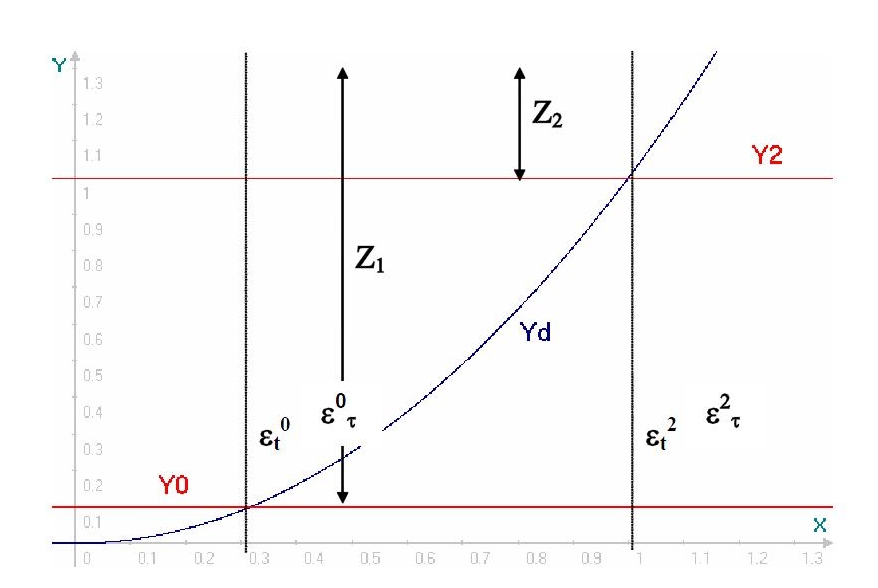
Figure 3.2-a: construction of threshold functions in terms of energy
The laws of evolution of the internal variables within the framework of the standard associated laws make it possible to obtain the derivative of the damage multiplier \({\lambda }_{D}\):
\(\stackrel{\text{.}}{D}\mathrm{=}{\stackrel{\text{.}}{\lambda }}_{D}\mathrm{\cdot }\frac{\mathrm{\partial }{\varphi }_{D}}{\mathrm{\partial }{Y}_{D}}\mathrm{=}{\stackrel{\text{.}}{\lambda }}_{D}\text{et}\stackrel{\text{.}}{z}\mathrm{=}{\stackrel{\text{.}}{\lambda }}_{D}\mathrm{\cdot }\frac{\mathrm{\partial }{\varphi }_{D}}{\mathrm{\partial }Z}\mathrm{=}\mathrm{-}{\stackrel{\text{.}}{\lambda }}_{D}\) eq 3.2-7
In addition, using the consistency condition, the expression of damage is obtained:
\({D}_{T}\mathrm{=}1\mathrm{-}\sqrt{\frac{{Y}_{\mathit{T1}}}{{Y}_{\mathit{DT}}}}\mathrm{\cdot }\text{exp}\left\{{A}_{{1}_{\mathit{DT}}}\mathrm{\cdot }{\left[\sqrt{\frac{2}{G}}\mathrm{\cdot }(\sqrt{{Y}_{\mathit{DT}}}\mathrm{-}\sqrt{{Y}_{\mathit{T1}}})\right]}^{{B}_{\mathrm{1DT}}}\right\}\mathrm{\ast }\)
\(\text{*}\left\{\frac{1}{1+{A}_{{2}_{\mathit{DT}}}\mathrm{\cdot }{\mathrm{\langle }{Y}_{\mathit{DT}}\mathrm{-}{Y}_{\mathit{T1}}\mathrm{\rangle }}_{+{{B}_{\mathrm{2DT}}}^{}}}\right\}\) eq 3.2-8
In this expression, we can identify the part that corresponds to the region of transition from \({A}_{{1}_{\mathrm{DT}}}\) small deformations to large slides with two parameters: and \({B}_{{1}_{\mathrm{DT}}}\), as well as the final damage part in mode 2, with the parameters \({A}_{{2}_{\mathrm{DT}}}\) and \({B}_{{2}_{\mathit{DT}}}\). It should be noted that the \(\mathrm{\langle }{Y}_{\mathit{DT}}\mathrm{-}{Y}_{\mathit{T1}}\mathrm{\rangle }\) relationship is managed by a Macaulay function, that is to say that this energy difference must always be positive or zero.
The functions that manage isotropic work hardening in the tangential direction are expressed as:
\({Z}_{\mathrm{T1}}={Y}_{\mathrm{DT}}-{Y}_{\mathrm{T1}};\) eq 3.2-9
\({Z}_{\mathit{T2}}\mathrm{=}\mathrm{\{}\begin{array}{cc}\mathrm{0,}& \text{si}{Y}_{\mathit{T1}}<{Y}_{\mathit{DT}}\mathrm{\le }{Y}_{\mathit{T2}}\\ {Y}_{\mathit{DT}}\mathrm{-}{Y}_{\mathit{T2}},& \text{si}{Y}_{\mathit{T2}}<{Y}_{\mathit{DT}}\end{array}\) eq 3.2-10
From these expressions, it can be noted that \({\mathrm{\Zeta }}_{\mathrm{T2}}\) is not taken into account in the transition region from small deformations to large slides.
3.3. Analysis of damage in the normal direction#
The two most important mechanisms that can occur in the normal direction are the detachment between the concrete and the steel bars, and the penetration of the reinforcement into the concrete body. These two conditions can be interpreted respectively as crack opening or closing, and can be described by a particular law of behavior in the normal direction decoupled from tangential behavior.
In order to simplify the resolution for compression between surfaces, we decided to allow a small penetration between them, which implies that \({\mathrm{\varepsilon }}_{N}\le 0\), and by adopting a law of elastic behavior, we will have:
\({\mathrm{\sigma }}_{N}=\begin{array}{ccc}E\cdot {\langle {\mathrm{\varepsilon }}_{N}\rangle }^{-}& \text{si}& {\mathrm{\varepsilon }}_{N}\le 0\end{array}\) eq 3.3-1
The case of interface decohesion can be described by damaging behavior in the normal direction, i.e.:
\({\mathrm{\sigma }}_{N}=\begin{array}{ccc}(1-{D}_{N})\cdot E\cdot {\langle {\mathrm{\varepsilon }}_{N}\rangle }^{+}& \text{si}& {\mathrm{\varepsilon }}_{N}>0\end{array}\) eq 3.3-2
with \({D}_{N}\) scalar variable of damage in the normal direction, calculated with the following expression:
\({D}_{N}\mathrm{=}\mathrm{\{}\begin{array}{ccc}0& \text{si}& {\varepsilon }_{N}\mathrm{\le }{\varepsilon }_{N}^{1}\\ & & \\ \frac{1}{1+{A}_{\mathit{DN}}\mathrm{\cdot }{\mathrm{\langle }{Y}_{\mathit{DN}}\mathrm{-}{Y}_{\mathit{N1}}\mathrm{\rangle }}_{+{{B}_{\mathit{DN}}}^{}}}& \text{si}& {\varepsilon }_{N}^{1}<{\varepsilon }_{N}\end{array}\) eq 3.3-3
In this expression, two material parameters, \({A}_{\mathit{DN}}\) and \({B}_{\mathit{DN}}\), control decohesion through tensile damage to concrete. Moreover, \({Y}_{\mathit{N1}}\) is the damage threshold defined in terms of energy, equivalent to the elastic threshold in the normal direction \({Y}_{\text{elas}}{\mathrm{\mid }}_{N}\) and which is expressed as:
\({Y}_{\mathit{N1}}\mathrm{=}{Y}_{\text{elas}}{\mathrm{\mid }}_{N}\mathrm{=}\frac{1}{2}{\varepsilon }_{N}^{1}\mathrm{\cdot }E\mathrm{\cdot }{\varepsilon }_{N}^{1}\) eq 3.3-4
\({\varepsilon }_{N}^{1}\) being the perfect adhesion limit deformation, which corresponds to the limiting deformation of concrete under tension before the initialization of the damage. It should be mentioned that when the detachment — or crack opening — reaches the maximum value of the tensile strength, no shear force should be transmitted between the two materials: this is the only condition in which the scalar variable of damage in the tangential direction becomes 1 due to damage in the normal direction
3.4. Analysis of the contribution of sliding crack friction#
As far as the « sliding » part of the formulation is concerned, it is assumed that it has a pseudoplastic behavior, with non-linear kinematic work hardening. Originally introduced by Armstrong & Frederick, 1966, cf. [bib1], nonlinear kinematic work hardening allows the formulation to overcome the main disadvantage of Prager’s kinematic work hardening law, namely, the linearity of state law that relates the forces associated with kinematic work hardening. Here, the nonlinear terms are added in the dissipation potential. The sliding criterion takes the classical form of the Drucker-Prager threshold function, which takes into account the effect of radial confinement on sliding:
\({\varphi }_{f}\mathrm{=}\mathrm{\mid }{\sigma }_{T}^{f}\mathrm{-}X\mathrm{\mid }+c\mathrm{\cdot }{I}_{1}\mathrm{\le }0\) eq 3.4-1
Here \(X\) is the recall constraint, \(c\) is a parameter linked to the material, reflecting the influence of confinement, while \({I}_{1}\) corresponds to the first invariant of the stress tensor, which for our case is expressed as:
\({I}_{1}\mathrm{=}\frac{1}{3}\text{Tr}\left[\sigma \right]\mathrm{=}\frac{1}{3}{\sigma }_{N}\) eq 3.4-2
Moreover, the initial threshold for slippage is 0. In addition, by considering the principle of maximum plastic dissipation, the laws of evolution can be derived from the expression of plastic potential which is:
\({\mathrm{\varphi }}_{f}^{p}=\mid {\mathrm{\sigma }}_{T}^{f}-\mathrm{\Khi }\mid +c\cdot {I}_{1}+\frac{3}{4}\cdot a\cdot {\mathrm{\Khi }}^{2}\) eq 3.4-3
Where \(a\) is a material parameter. It should be mentioned that the term quadratic in \(\mathrm{\Khi }\) makes it possible to introduce the non-linearity of kinematic work hardening. The laws of evolution for sliding deformation as well as for kinematic work hardening take the following forms:
\(\stackrel{\text{.}}{{\varepsilon }_{T}^{f}}\mathrm{=}{\stackrel{\text{.}}{\lambda }}_{f}\mathrm{\cdot }\frac{\mathrm{\partial }{\varphi }_{f}^{p}}{\mathrm{\partial }{\sigma }_{T}^{f}}\text{et}\stackrel{\text{.}}{\alpha }\mathrm{=}{\stackrel{\text{.}}{\lambda }}_{f}\mathrm{\cdot }\frac{\mathrm{\partial }{\varphi }_{f}^{p}}{\mathrm{\partial }X}\) eq 3.4-4
The slippage multiplier \(\dot{{\lambda }_{f}}\) is calculated numerically by imposing the consistency condition.
3.5. Summary of equations#
Here we show a summary of the equations that constitute the law of behavior of the steel-concrete bond:
Helmholtz Free Energy |
\(\begin{array}{c}\rho \text{.}\psi \mathrm{=}\frac{1}{2}\mathrm{[}{\mathrm{\langle }{\varepsilon }_{N}\mathrm{\rangle }}^{\mathrm{-}}E{\mathrm{\langle }{\varepsilon }_{N}\mathrm{\rangle }}^{\mathrm{-}}+{\mathrm{\langle }{\varepsilon }_{N}\mathrm{\rangle }}^{+}E\text{.}(1\mathrm{-}{D}_{N}){\mathrm{\langle }{\varepsilon }_{N}\mathrm{\rangle }}^{+}\\ +{\varepsilon }_{T}G(1\mathrm{-}{D}_{T}){\varepsilon }_{T}+({\varepsilon }_{T}\mathrm{-}{\varepsilon }_{T}^{f})G\text{.}{D}_{T}({\varepsilon }_{T}\mathrm{-}{\varepsilon }_{T}^{f})+\gamma {\alpha }^{2}\mathrm{]}+H(z)\end{array}\) |
Threshold function |
\(\begin{array}{c}{\varphi }_{\mathit{DT}}\mathrm{=}{Y}_{\mathit{DT}}\mathrm{-}({Y}_{\mathit{T1}}+{Z}_{T})\mathrm{\le }0;\\ {\varphi }_{f}\mathrm{=}\mathrm{\mid }{\sigma }_{T}^{f}\mathrm{-}X\mathrm{\mid }+c\text{.}{I}_{1}\mathrm{\le }0\end{array}\) |
State Laws |
\(\begin{array}{c}{\sigma }_{N}\mathrm{=}\mathrm{\{}\begin{array}{cc}E\text{.}{\varepsilon }_{N}& \text{si}{\varepsilon }_{N}\mathrm{\le }0\\ (1\mathrm{-}{D}_{N})\text{.}E\text{.}{\varepsilon }_{N}& \text{si}{\varepsilon }_{N}>0\end{array};\\ {\sigma }_{T}\mathrm{=}G(1\mathrm{-}{D}_{T}){\varepsilon }_{T}+G\text{.}{D}_{T}({\varepsilon }_{T}\mathrm{-}{\varepsilon }_{T}^{f});\\ {\sigma }_{T}^{f}\mathrm{=}G\text{.}{D}_{T}({\varepsilon }_{T}\mathrm{-}{\varepsilon }_{T}^{f})\end{array}\) |
Dissipation |
\(\begin{array}{c}\mathrm{-}Y\mathrm{=}\mathrm{-}\rho \frac{\mathrm{\partial }\psi }{\mathrm{\partial }D}\mathrm{=}\mathrm{-}({Y}_{D}+{Y}_{f});\\ X\mathrm{=}\rho \frac{\mathrm{\partial }\psi }{\mathrm{\partial }\alpha }\mathrm{=}\gamma \alpha ;\\ Z\mathrm{=}\rho \frac{\mathrm{\partial }\psi }{\mathrm{\partial }z}\mathrm{=}{H}^{\text{'}}(z)\end{array}\) |
Laws of evolution |
\(\begin{array}{c}\dot{D}\mathrm{=}{\dot{\lambda }}_{D}\text{.}\frac{\mathrm{\partial }{\varphi }_{D}}{\mathrm{\partial }{Y}_{D}}\mathrm{=}{\dot{\lambda }}_{D};\dot{z}\mathrm{=}{\dot{\lambda }}_{D}\text{.}\frac{\mathrm{\partial }{\varphi }_{D}}{\mathrm{\partial }Z}\mathrm{=}\mathrm{-}{\dot{\lambda }}_{D};\\ {\dot{\varepsilon }}_{T}^{f}\mathrm{=}{\dot{\lambda }}_{f}\text{.}\frac{\mathrm{\partial }{\varphi }_{f}^{p}}{\mathrm{\partial }{\sigma }_{T}^{f}};\dot{\alpha }\mathrm{=}{\dot{\lambda }}_{f}\text{.}\frac{\mathrm{\partial }{\varphi }_{f}^{p}}{\mathrm{\partial }X}\end{array}\) |
3.6. Tangent matrix expression#
In order to ensure the robustness and efficiency of the model in numerical implantation and for the global analysis of massive structures, it is necessary to calculate the tangent matrix, which can be determined from the following expression:
\(\stackrel{\text{.}}{{\sigma }_{T}}\mathrm{=}H\mathrm{\cdot }\stackrel{\text{.}}{{\varepsilon }_{T}}\) eq 3.6-1
After some analytical calculations, we can deduce the expression for the tangent module using the consistency condition and the respective laws of evolution:
\(H=\frac{G\cdot (1-(\partial g({\mathrm{\varepsilon }}_{T})/\partial {\mathrm{\varepsilon }}_{T})\cdot {\mathrm{\varepsilon }}_{T}^{f})}{1+G\cdot {D}_{T}(\frac{(\partial {\mathrm{\varphi }}_{f}/\partial {\mathrm{\sigma }}_{T})\cdot (\partial {\mathrm{\varphi }}_{f}^{p}/\partial {\mathrm{\sigma }}_{T})}{(\partial {\mathrm{\varphi }}_{f}/\partial \mathrm{\Khi })({\partial }^{2}\mathrm{\rho }\mathrm{\psi }/\partial {\mathrm{\alpha }}^{2})(\partial {\mathrm{\varphi }}_{f}^{p}/\partial \mathrm{\Khi })})}\) eq 3.6-2
With
\(\frac{\mathrm{\partial }g({\varepsilon }_{T})}{\mathrm{\partial }{\varepsilon }_{T}}\mathrm{=}\frac{\mathrm{\partial }{D}_{T}}{\mathrm{\partial }{Y}_{\mathit{DT}}}\mathrm{\cdot }\frac{\mathrm{\partial }{Y}_{\mathit{DT}}}{\mathrm{\partial }{\varepsilon }_{T}}\mathrm{=}\left[\frac{f\mathrm{\cdot }g\mathrm{\cdot }h\text{'}\mathrm{-}f\text{'}\mathrm{\cdot }g\mathrm{\cdot }h\mathrm{-}f\mathrm{\cdot }g\text{'}\mathrm{\cdot }h}{{h}^{2}}\right]\mathrm{\cdot }G\mathrm{\cdot }{\varepsilon }_{T}\) eq 3.6-3
Where \(f,g\) and \(h\) are the following functions, obtained using [éq 3.2-8]:
\(f\mathrm{=}\sqrt{\frac{{Y}_{\mathit{T1}}}{{Y}_{\mathit{DT}}}}\) eq 3.6-4
\(g\mathrm{=}\text{exp}\left\{{A}_{{1}_{\mathit{DT}}}\mathrm{\cdot }{\left[\sqrt{\frac{2}{G}}\mathrm{\cdot }(\sqrt{{Y}_{\mathit{DT}}}\mathrm{-}\sqrt{{Y}_{\mathit{T1}}})\right]}^{{B}_{\mathrm{1DT}}}\right\}\) eq 3.6-5
\(h\mathrm{=}1+{A}_{{2}_{\mathit{DT}}}\mathrm{\cdot }{\mathrm{\langle }{Y}_{\mathit{DT}}\mathrm{-}{Y}_{\mathit{T1}}\mathrm{\rangle }}_{+{{B}_{\mathrm{2DT}}}^{}}\) eq 3.6-6
Note:
In practice in Aster, the tangent matrix has not been implemented, only the secant matrix is used either \(H=(\begin{array}{cc}E(1-{D}_{N})& 0\\ 0& G(1-{D}_{T})\end{array})\).