3. Discretization of the thermo-hydration problem

3.1. Choosing the resolution method

The method chosen consists in solving the non-linear equation [] globally by taking advantage of the non-linear thermal algorithm of*Code_Aster* and locally solving the equation [] which represents the law of evolution of a kind of internal variable representing the degree of hydration, this law being expressed by a function of the thermal state of the system. Indeed, there is no differential operator in space for the variable \(\xi\) in the equations and therefore no need for a finite element. The relationship [] represents a local law as in plasticity. The same number of degrees of freedom as for conventional thermal engineering is then maintained. Such a decoupled process nevertheless involves the calculation of the same quantities several times. Indeed, let’s say \(\xi\) is discretized at element nodes. Let us consider the example schematized by the [].

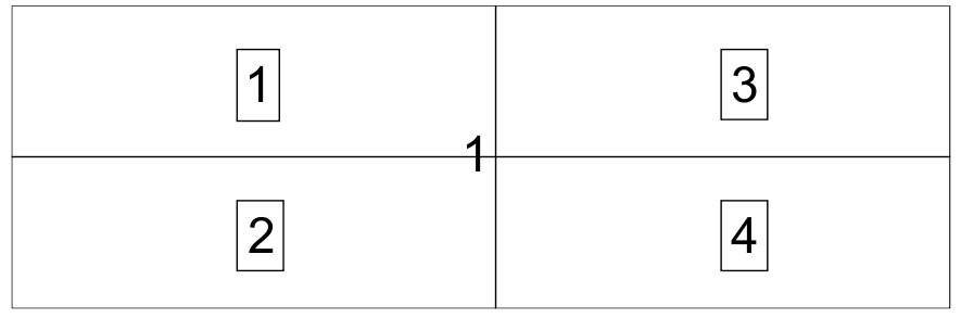
Figure 3.1-1

On the 1 node, the evolution equation [] will be integrated four times. A possible solution would have been for local calculations to be able to be done on fields at the nodes (concept Aster CHAM_NO) and not on fields of nodes by element (concept Aster CHAM_ELEM, option ELNO), which is currently impossible.

The solution that was finally adopted consists in calculating \(\xi\) at the gauss points of the element, which is all the more natural since for mechanical calculation the Young’s modulus depends explicitly on \(\xi\). However, this generates a lot of local calculations except to greatly under-integrate the finite element. For example, if you consider a mesh with \(N\) hexahedral elements with 20 knots, there are roughly \(\mathrm{4N}\) nodes and \(\mathrm{27N}\) Gauss points.

3.2. Resolution algorithm

The weak formulation of equation [] is written as follows:

|:math: begin {array} {c} {c} {mathrm {int}} _ {omega}dot {beta} (T)mathrm {cdot} {T} ^ {text {*}} ^ {text {*}}} domega + {mathrm {int}} _ {omega}lambda (T)mathrm {nabla}} ^ {text {*}}} domega + {mathrm {int}}} _ {omega}lambda (T)mathrm {nabla} {*}} thrm {cdot}mathrm {nabla} {T} {T} ^ {text {*}} domegamathrm {int}} _ {omega} smathrm {cdot} {T} {T} ^ {text {*}}} domega + {mathrm {int}}} _ {omega}} smathrm {int}} smathrm {omega} smathrm {cdot} {T} {T} ^ {text {*}}} domega + {mathrm {int}}} _ {omega}} (xi) {e} ^ {mathrm {-}frac {{E}}frac {{E} _ {a}} {mathit {RT}}}mathrm {cdot} {T} ^ {text {*}} ^ {*}} domega + {mathrm {*}}} domega + {mathrm {int}} _ {gamma}Phimathrm {cdot} {T} {T} {T}} ^ {*}} dOmega + {mathrm {int}}} {*}} dGamma\\mathrm {forall} {forall} {T} ^ {text {*}}end {array} | eq 3.2-1 | +————————————————————————————————————————————————————————————————————————————————————————————————————————————————————————————————————————————————————————————————————————————–+———-+

The development of thermohydration within the general nonlinear thermal algorithm in Code_Aster therefore consists in explicitly discretizing the term \({\mathrm{\int }}_{\Omega }QA(\xi ){e}^{\mathrm{-}\frac{{E}_{a}}{\mathit{RT}}}\mathrm{\cdot }{T}^{\text{*}}d\Omega\) in the second member.

By noting \({\xi }^{-},{T}^{-},{\xi }^{+},{T}^{+}\) respectively, the hydration and temperature variables at the beginning and at the end of the time step, we calculate at each Gauss point the quantity:

\(QA({\xi }^{\mathrm{-}}){e}^{\mathrm{-}\frac{{E}_{a}}{{\text{RT}}^{\mathrm{-}}}}\)

which is integrated directly into the second member. After each resolution of the current step, the variables are updated \(({\xi }^{+}={\xi }^{-},{T}^{+}={T}^{-})\). The convergence test is only active on temperature, the variable \(\xi\) not entering into the iterative Newton process used in nonlinear thermics. Taking hydration into account is in fact just taking into account a known heat source at the beginning of the time step. This purely explicit discretization therefore requires the use of sufficiently small time steps.