2. Law of behavior#
2.1. Theoretical writing#
If we want to take into account the reclosing effect, we must pay great attention to the continuity of the stresses as a function of the deformations (which is an indispensable condition for a law of behavior in a finite element calculation software), confer [bib1]. Indeed, if this effect is modelled too simplistically, the law of behavior is very likely to present a discontinuous response.
To take into account reclosing (i.e. the transition between traction and compression), it is necessary to start by finely describing what is called traction and compression, knowing that under tension (resp. compression) the crack will be considered « open » (resp. « closed »). A natural solution is to place yourself in a specific deformation frame. In such a coordinate system, elastic free energy is written (\(\lambda\) and \(\mu\) designating the Lamé coefficients):
\(\Phi (\varepsilon )\frac{\lambda }{2}{(\mathit{tr}\varepsilon )}^{2}+\mu \mathrm{\sum }_{i}{\varepsilon }_{i}^{2}\) eq 2.1-1
We can then define:
traction or volume compression, following the sign of \(t\varepsilon\),
traction or compression in each specific direction, following the sign of \({\varepsilon }_{i}\).
According to the following fairly reasonable principle - in a case of traction (« open crack »), we correct the elastic energy by a damage factor; in a case of compression (« closed crack »), we keep the expression of elastic energy -, the damagable free energy is written:
\(\Phi (\varepsilon ,d)=\frac{\lambda }{2}{(\mathrm{tr}\varepsilon )}^{2}(H(-\mathrm{tr}\varepsilon )+\frac{1-d}{1+\gamma d}H(\mathrm{tr}\varepsilon ))+\mu \sum _{i}{\varepsilon }_{i}^{2}(H(-{\varepsilon }_{i})+\frac{1-d}{1+\gamma d}H({\varepsilon }_{i}))\) eq 2.1-2
We notice that the free energy is continuous with each change of regime. It is even continuously differentiable with respect to deformations, since it is the sum of differentiable functions (function \({x}^{2}H(x)\) is differentiable) and the continuity of the partial derivatives at points \(t\varepsilon =0\) and \({\varepsilon }_{i}=0\) is immediate. The constraints are then explained (knowing that they will be continuous functions of deformations everywhere). As in elasticity, the natural stress coordinate system coincides with the deformation coordinate system, a result shown in the appendix.
We write the constraints in the proper coordinate system:
\({\sigma }_{\mathit{ii}}\mathrm{=}\lambda (\mathit{tr}\varepsilon )(H(\mathrm{-}\mathit{tr}\varepsilon )+\frac{1\mathrm{-}d}{1+\gamma d}H(\mathit{tr}\varepsilon ))+2\mu {\varepsilon }_{\mathit{ii}}(H(\mathrm{-}{\varepsilon }_{\mathit{ii}})+\frac{1\mathrm{-}d}{1+\gamma d}H({\varepsilon }_{\mathit{ii}}))\) eq 2.1-3
In this form, the continuity of the stresses with respect to the deformations is clear. The figure opposite shows the stress \({\sigma }_{11}\) in plane \(({\varepsilon }_{\mathrm{1,}}{\varepsilon }_{2})\) at constant damage (2D case, plane deformation). The effect of reclosing as well as the continuity of the stresses are clearly visible.
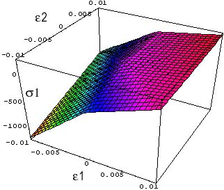
Figure 2-a: illustration of continuity.
The thermodynamic force \({F}^{d}\) associated with the internal damage variable is written as:
\({F}^{d}\mathrm{=}\mathrm{-}\frac{\mathrm{\partial }\Phi }{\mathrm{\partial }d}\mathrm{=}\frac{1+\gamma }{{(1+\gamma d)}^{2}}(\frac{\lambda }{2}{(\mathit{tr}\varepsilon )}^{2}H(\mathit{tr}\varepsilon )+\mu \mathrm{\sum }_{i}{\varepsilon }_{i}^{2}H({\varepsilon }_{i}))\) eq 2.1-4
The evolution of the damage remains to be defined. The schema used is that of generalized standard models. You have to define a criterion, which you take in the form of:
\(f({F}^{d})={F}^{d}(\varepsilon ,d)-k\) eq 2.1-5
where k defines the damage threshold. In order to take into account, at the level of the evolution of the damage, the confinement effect, threshold \(k\) depends on the state of deformation, in the form of:
\(k\mathrm{=}{k}_{0}\mathrm{-}{k}_{1}(\mathit{tr}\varepsilon )H(\mathrm{-}\mathit{tr}\varepsilon )\) eq 2.1-6
We are committed to staying in the field:
\(f({F}^{d})\mathrm{\le }0\) eq 2.1-7
The evolution of the damage variable is then determined by the Kuhn-Tucker conditions:
\(\mathrm{\{}\begin{array}{c}\dot{d}\mathrm{=}0\mathit{pour}f<0\\ \dot{d}\mathrm{\ge }0\mathit{pour}f\mathrm{=}0\end{array}\) eq 2.1-8
For uniaxial stress, the resulting curve is shown in FIG. 2-b, for two confinement values (see paragraph 2.3.2.2). In compression, the behavior remains approximately linear, which only represents the behavior of the material up to 3-4 times the value of the (uniaxial) tensile strength, here \(\mathit{SYT}\). It is clear that the use of the law is then indicated as long as one stays within this limit. In FIG. 2-b, the test piece is first loaded with traction and is thus damaged. Then it is unloaded and subsequently loaded into compression in the same direction. We will therefore notice the resumption of stiffness under compression (crack closure).
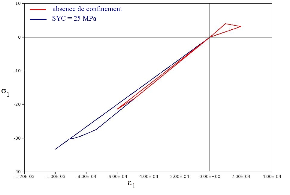
Figure 2-b: response to uniaxial stress.
It can be seen that in a pure uniaxial damaging load (\(\dot{d}\ge 0\)), the thermodynamic force is expressed: \({F}^{d}(d)=-E\frac{{\varepsilon }^{2}\mathrm{.}{\xi }_{,d}(d)}{2}\), having noted \(\xi (d)=\frac{1-d}{1+\gamma d}\). The consistency condition is then written as:
\(\dot{f}=-E\varepsilon \dot{\varepsilon }{\xi }_{,d}-E\frac{{\varepsilon }^{2}\dot{d}{\xi }_{,\mathrm{dd}}}{2}=0\) eq 2.1-9
Hence: \(\dot{d}=-\frac{2\dot{\varepsilon }{\xi }_{,d}}{\varepsilon {\xi }_{,\mathrm{dd}}}\) and therefore the law of pure uniaxial damaging membrane charge is:
\(\dot{\sigma }=E({\xi }_{,d}\dot{d}\varepsilon +{\xi }_{\dot{\varepsilon }})=E\dot{\varepsilon }(\xi -2\frac{{\xi }_{,d}^{2}}{{\xi }_{,\mathrm{dd}}})=\frac{-E}{\gamma }\dot{\varepsilon }\) eq 2.1-10
This makes it possible to interpret the role of the parameter \(\gamma\): the slope being constant, which is the justification for the algebraic form of the function \(\xi\).
Note:
From a formal point of view, generalized standard materials are characterized by a dissipation potential positively homogeneous function of degree 1, Legendre-Fenchel transform of the function indicative of the reversibility domain, which is therefore valid here:
\(\Delta (\dot{d})\mathrm{=}\underset{{F}^{d}\mathrm{/}f({F}^{d})\mathrm{\le }0}{\text{sup}}{F}^{d}\dot{d}\mathrm{=}k\dot{d}+{I}_{{\mathit{IR}}^{\text{+}}}(\dot{d})\) eq 2.1-11
Note the presence of an indicator function relating to \(\dot{d}\), which ensures that damage is increasing.
It is still necessary to take into account the fact that the damage is increased by 1. From an intuitive point of view, it seems easy. To keep writing fully compatible with the generalized standard formalism, it suffices to introduce a function indicative of the admissible domain into the expression of free energy:
\(\begin{array}{cc}\Phi (\varepsilon ,d)\mathrm{=}& \frac{\lambda }{2}{(\mathit{tr}\varepsilon )}^{2}(H(\mathrm{-}\mathit{tr}\varepsilon )+\frac{1\mathrm{-}d}{1+\gamma d}H(\mathit{tr}\varepsilon ))+\\ & \mu \mathrm{\sum }_{i}{\varepsilon }_{i}^{2}(H(\mathrm{-}{\varepsilon }_{i})+\frac{1\mathrm{-}d}{1+\gamma d}H({\varepsilon }_{i}))+{I}_{\left]\mathrm{-}\mathrm{\infty };1\right]}(d)\end{array}\) eq 2.1-12
The introduction of this indicator function prevents the damage from exceeding 1, in fact, for \(d\mathrm{=}1\), \({F}^{d}\mathrm{=}\frac{\mathrm{-}\mathrm{\partial }f}{\mathrm{\partial }d}\mathrm{=}\mathrm{-}\mathrm{\infty }\), and the damage no longer evolves.
2.2. Taking into account shrinkage and temperature#
The law of behavior takes into account a possible shrinkage due to desiccation, a possible endogenous shrinkage and a possible thermal deformation. The deformation \(\varepsilon\) that is referred to in this document then being the « elastic deformation » \(\tilde{\varepsilon }\mathrm{=}\varepsilon \mathrm{-}{\varepsilon }^{\mathit{th}}\mathrm{-}{\varepsilon }^{\mathit{rd}}\mathrm{-}{\varepsilon }^{\text{re}}\).
On the other hand, the material parameters that will be discussed in the next paragraph are considered to be constants (in particular, they cannot be temperature dependent, in the current state of development)
2.3. Identifying parameters#
The parameters of the law of behavior are 4 or 5 in number (see next paragraphs). They are typically provided in operator DEFI_MATERIAU.
2.3.1. Elastic parameters#
These are the simplest: they are the two classical parameters, Young’s modulus and Poisson’s ratio, provided under the ELAS or ELAS_FO keyword of DEFI_MATERIAU.
2.3.2. Damage parameters#
Depending on whether the user wants to use the threshold dependence with confinement or not, 2 or 3 parameters must be provided to control the damage law.
2.3.2.1. Use without dependence on confinement#
In this case, the parameter \({k}_{1}\) is considered to be zero. It should be noted that the state of compression of concrete must remain moderate for the law to remain valid (compressive stress of the order of a few times the stress at peak tension, in absolute value).
The user must enter, under the BETON_ECRO_LINE DEFI_MATERIAU keyword, the values of:
SYT: limit of the stress in simple tension,
D_ SIGM_EPSI: slope of the post-peak curve under traction.
The value of SYC is then automatically calculated to have k1=0 and takes its minimum value, i.e.:
\(\mathit{SYC}=\mathit{SYT}\sqrt{\frac{1+\nu -2{\nu }^{2}}{2{\nu }^{2}}}\)
2.3.2.2. Use with dependence on confinement#
In this case, the dependence on confinement allows concrete to maintain realistic compression behavior up to the order of magnitude of occurrence of non-linearity in compression, given by SYC, Cf. below (classically, a compressive stress of the order of ten times the stress at the peak of tension, in absolute value).
The user must enter, under the BETON_ECRO_LINE DEFI_MATERIAU keyword, the values of:
SYT: limit of the stress in simple tension,
SYC: stress limit in simple compression,
D_ SIGM_EPSI: slope of the post-peak curve under traction.
Figure 2-b shows the behavior with two values of confinement. Increasing the SYC parameter has the effect of extending the linear behavior of the material.
2.3.2.3. Transition from « user » values to « model » values#
For information, we obtain the values of \(\gamma\), \({k}_{0}\) and possibly \({k}_{1}\) (if the user has entered SYC) by the following formulas, cf. [éq 2.1-10]:
\(\gamma \mathrm{=}\frac{\mathrm{-}E}{\text{D\_SIGM\_EPSI}}\)
\({k}_{0}={(\mathrm{SYT})}^{2}(\frac{1+\gamma }{2E})(\frac{1+\nu -2{\nu }^{2}}{1+\nu })\)
\({k}_{1}=\mathrm{SYC}\frac{(1+\gamma ){\nu }^{2}}{(1+\nu )(1-2\nu )}-{k}_{0}\frac{E}{(1-2\nu )(\mathrm{SYC})}\)
2.4. Digital integration#
Two points need to be resolved before implementing the model: the first concerns the evaluation of the damage; the second consists in calculating the tangent matrix, a calculation made a little more difficult than usual by the transition to a proper deformation coordinate system.
We place ourselves here in the framework of the implicit integration of laws of behavior. The dependence of the criterion on the confinement [éq 2.1-6] is taken into account in explicit form, i.e. the threshold \(k\) is entirely determined by the deformation state of the previous step, in order to simplify the integration of the model.
2.4.1. Damage assessment#
As we will see, a simple scalar equation makes it possible to obtain the damage, which makes it possible to avoid recourse to iterative methods.
We note \({d}^{\text{-}}\) the damage at the previous step and \({d}^{\text{+}}\) the evaluation of the damage at the current step at the current iteration which will be the damage at the current step when convergence is reached. The easiest way to assess the damage of the current iteration is to assume that the criterion is reached at the current moment, which results in:
\(f({F}^{d})\mathrm{=}0\mathrm{\Rightarrow }\frac{1+\nu }{{(1+\gamma d)}^{2}}(\frac{\lambda }{2}{(\mathit{tr}\varepsilon )}^{2}H(\mathit{tr}\varepsilon )+\mu \mathrm{\sum }_{i}{\varepsilon }_{i}^{2}H({\varepsilon }_{i}))\mathrm{=}k\) eq 2.4.1-1
This results in:
\({d}^{\mathit{test}}\mathrm{=}\frac{1}{\gamma }(\sqrt{\frac{1+\gamma }{k}(\frac{\lambda }{2}{(\mathit{tr}\varepsilon )}^{2}H(\mathit{tr}\varepsilon )+\mu \mathrm{\sum }_{i}{\varepsilon }_{i}^{2}H({\varepsilon }_{i}))}\mathrm{-}1)\) eq 2.4.1-2
3 cases occur:
\({d}^{\mathrm{test}}\le {d}^{\text{-}}\): this means that at the current moment, the criterion is not met, we conclude that \({d}^{\text{+}}={d}^{\text{-}}\),
\({d}^{\text{-}}\le {d}^{\mathrm{test}}\le 1\): the criterion is therefore met, the consistency condition implies \({d}^{\text{+}}={d}^{\mathrm{test}}\),
\({d}^{\mathrm{test}}\ge 1\): the material is then ruined at this point, hence \({d}^{\text{+}}\mathrm{=}1\).
2.4.2. Calculation of the tangent matrix#
The tangent matrix is the sum of two terms, the first expressing the stress-strain relationship at constant damage, the second being derived from condition \(f\mathrm{=}0\). In fact, we can write:
\(\frac{\mathrm{\partial }{\sigma }_{\mathit{ij}}}{\mathrm{\partial }{\varepsilon }_{\mathit{kl}}}\mathrm{=}{\left\{\frac{\mathrm{\partial }{\sigma }_{\mathit{ij}}}{\mathrm{\partial }{\varepsilon }_{\mathit{kl}}}\right\}}_{d\mathrm{=}{c}^{\mathit{te}}}+\frac{\mathrm{\partial }{\sigma }_{\mathit{ij}}}{\mathrm{\partial }d}{\left\{\frac{\mathrm{\partial }d}{\mathrm{\partial }{\varepsilon }_{\mathit{kl}}}\right\}}_{f\mathrm{=}0}\) eq 2.4.2-1
If the user requests the calculation with a tangent matrix (Cf. documentation from STAT_NON_LINE, [U4.51.03]), the law of behavior provides the expression given by [éq 2.4.2-1]. On the other hand, if the user requests the calculation with the discharge matrix, the law of behavior provides the secant matrix, that is, the first term on the right-hand side of [éq 2.4.2-1].
2.4.2.1. Tangent matrix with constant damage#
As we pointed out earlier, calculating the tangent matrix is a bit tricky because of the way the model is written in the proper deformation coordinate system. Thus, it is easy to know the tangent matrix with constant damage in the natural deformation coordinate system, and what we are looking for is this same tangent matrix in the global coordinate system.
In the case where the damage does not change, in the specific deformation coordinate system, the desired matrix expresses a simple relationship of degraded elasticity:
\({\left\{\frac{\delta \tilde{{\sigma }_{i}}}{\delta \tilde{{\varepsilon }_{j}}}\right\}}_{d\mathrm{=}{C}^{\mathit{te}}}\mathrm{=}\lambda (H(\mathrm{-}\mathit{tr}\varepsilon )+\frac{1\mathrm{-}d}{1+\gamma d}H(\mathit{tr}\varepsilon ))+2\mu {\delta }_{\mathit{ij}}(H(\mathrm{-}{\varepsilon }_{j})+\frac{1\mathrm{-}d}{1+\gamma d}H({\varepsilon }_{j}))\) eq 2.4.2.1-1
It is now necessary to express the transition from the global coordinate system to the natural deformation coordinate system, at least in the case where the deformation eigenvalues are different. Since the tangent matrix is only necessary for numeric resolution algorithms (Newton diagram), it will be possible, when calculating the tangent matrix (and only in this case), to numerically disturb any identical eigenvalues (in order to make them distinct). In particular, it will be noted that this makes it possible, with zero damage, to recover the elastic stiffness matrix.
We denote with a tilde the tensors in the natural deformation coordinate system (which, as we recall, is also the natural stress coordinate system). By definition, by noting \({U}_{i}\) the eigenvector associated with the i-th eigenvalue, the matrix change of base \(Q\mathrm{=}({U}_{1}{U}_{2}{U}_{3})\), we have:
\(\sigma \mathrm{=}Q\tilde{\sigma }{Q}^{T}\mathrm{\Rightarrow }\delta {\sigma }_{\mathit{ij}}\mathrm{=}{Q}_{\text{im}}{Q}_{\text{jm}}\delta \tilde{{\sigma }_{m}}+\delta {Q}_{\text{im}}{Q}_{\text{jm}}\tilde{{\sigma }_{m}}+{Q}_{\text{im}}\delta {Q}_{\text{jm}}\tilde{{\sigma }_{m}}\)
In the case where the deformation eigenvalues are distinct, the evolution of the eigenvectors and eigenvalues is given by (see above [§2]):
\(\dot{{U}_{j}}\mathrm{.}{U}_{k}\mathrm{=}\frac{\dot{\tilde{{\varepsilon }_{\mathit{jk}}}}}{\tilde{{\varepsilon }_{j}}\mathrm{-}\tilde{{\varepsilon }_{k}}}\) for \(j\mathrm{\ne }k\) eq 2.4.2.1-2
\(\dot{\tilde{{\varepsilon }_{i}}}\mathrm{=}\dot{\tilde{{\varepsilon }_{\mathit{ii}}}}\) for \(j\mathrm{\ne }k\) eq 2.4.2.1-3
We can easily deduce \(\delta Q\):
\(\delta {Q}_{\mathit{ij}}\mathrm{=}\mathrm{\sum }_{k\mathrm{\ne }j}\frac{\delta \tilde{{\varepsilon }_{\mathit{jk}}}}{\tilde{{\varepsilon }_{j}}\mathrm{-}\tilde{{\varepsilon }_{k}}}{({U}_{k})}_{i}\mathrm{=}\mathrm{\sum }_{k\mathrm{\ne }j}\frac{\delta \tilde{{\varepsilon }_{\mathit{jk}}}}{\tilde{{\varepsilon }_{j}}\mathrm{-}\tilde{{\varepsilon }_{k}}}{Q}_{\mathit{ik}}\) eq 2.4.2.1-4
Then using (the last expression only used to obtain a clearly symmetric matrix):
\(\delta \tilde{{\varepsilon }_{\mathit{ij}}}\mathrm{=}{Q}_{\mathit{ki}}{Q}_{\mathit{lj}}{\varepsilon }_{\mathit{kl}}\mathrm{=}\frac{1}{2}({Q}_{\mathit{ki}}{Q}_{\mathit{lj}}+{Q}_{\mathit{li}}{Q}_{\mathit{kj}}){\varepsilon }_{\mathit{kl}}\)
So we get:

eq 2.4.2.1-5
The tangent matrix with constant damage is therefore written as:
\({A}_{\mathit{ijkl}}\mathrm{=}\frac{\mathrm{\partial }{\sigma }_{\mathit{ij}}}{\mathrm{\partial }{\varepsilon }_{\mathit{kl}}}\mathrm{=}\mathrm{\sum }_{m,n}{Q}_{\text{im}}{Q}_{\text{jm}}{Q}_{\text{kn}}{Q}_{\text{ln}}{\left\{\frac{\delta \tilde{{\sigma }_{m}}}{\delta \tilde{{\varepsilon }_{n}}}\right\}}_{d\mathrm{=}{C}^{\mathit{te}}}+\frac{1}{2}\mathrm{\sum }_{m,n\mathrm{:}n\mathrm{\ne }m}(\frac{({Q}_{\text{km}}{Q}_{\text{ln}}+{Q}_{\text{lm}}{Q}_{\text{kn}})({Q}_{\text{in}}{Q}_{\text{jm}}{Q}_{\text{jn}}{Q}_{\text{im}})}{\tilde{{\varepsilon }_{n}}\mathrm{-}\tilde{{\varepsilon }_{m}}})\tilde{{\sigma }_{m}}\) eq 2.4.2.1-6
2.4.2.2. Term of the tangent matrix due to the evolution of the damage#
The expression to be evaluated is written as:
\(\frac{\mathrm{\partial }{\sigma }_{\mathit{ij}}}{\mathrm{\partial }d}{\left\{\frac{\mathrm{\partial }d}{\mathrm{\partial }{\varepsilon }_{\mathit{kl}}}\right\}}_{f\mathrm{=}0}\) eq 2.4.2.2-1
We write the equation [éq 2.4.1-1] in the form:
\(\frac{1+\gamma }{{(1+\gamma d)}^{2}}\left[W(\varepsilon )\right]\mathrm{=}k\) eq 2.4.2.2-2
with: \(W(\varepsilon )\mathrm{=}\frac{\lambda }{2}{(\mathit{tr}\varepsilon )}^{2}H(\mathit{tr}\varepsilon )+\mu \mathrm{\sum }_{i}{\varepsilon }_{i}^{2}H({\varepsilon }_{i})\).
In differentiating this expression, it comes:
\(\mathrm{-}\frac{2\gamma (1+\gamma )}{{(1+\gamma d)}^{3}}W(\varepsilon )\delta d+\frac{1+\gamma }{{(1+\gamma d)}^{2}}{\sigma }^{\mathit{el}}\mathrm{\cdot }\delta \varepsilon \mathrm{=}0\) eq 2.4.2.2-3
with: \({\sigma }^{\mathit{el}}\mathrm{=}\frac{\mathrm{\partial }W}{\mathrm{\partial }\varepsilon }\)
The following equation is then used:
\(\frac{\mathrm{\partial }\sigma }{\mathrm{\partial }d}\mathrm{=}\mathrm{-}\frac{1+\gamma }{{(1+\gamma d)}^{2}}{\sigma }^{\mathit{el}}\) eq 2.4.2.2-4
We conclude:
\({\left\{\frac{\mathrm{\partial }{\sigma }_{\mathit{ij}}}{\mathrm{\partial }{\varepsilon }_{\mathit{kl}}}\right\}}_{f\mathrm{=}0}\mathrm{=}\mathrm{-}\frac{1+\gamma }{2\gamma (1+\gamma d)W(\varepsilon )}{\sigma }_{\mathit{ij}}^{\mathit{el}}{\sigma }_{\mathit{kl}}^{\mathit{el}}\) eq 2.4.2.2-5
2.4.3. Case of completely damaged material#
In the case of completely damaged material, \(d\mathrm{=}1\), the stiffness of the material point may cancel out. This is not a problem for the stress; on the other hand, it can result in zero pivots in the stiffness matrix. To overcome this difficulty, it is possible to define a minimum stiffness for the tangent matrix or the discharge matrix. This minimum stiffness does not affect the damage value (which can reach 1) or the stress (which can reach 0).
To maintain reasonable conditioning of the stiffness matrix, the minimum stiffness is taken to \({10}^{\mathrm{-}5}\) of the initial stiffness. A \(\chi\) flag specifies the behavior during the current time step:
\(\chi \mathrm{=}0\): no evolution of the damage during the step,
\(\chi =1\): evolution of damage during the step,
\(\chi =2\): saturated damage

.
2.5. Description of internal variables#
The model has two internal variables:
\(\mathrm{VI}(1)\): damage \(d\),
\(\mathit{VI}(2)\): indicator \(\chi\)