3. Reversibility domain and threshold functions

3.1. Allure of the domain and the reversibility thresholds

The reversibility domain is the domain of stress space within which stress paths are reversible. In the space of the main constraints \(({\sigma }_{\mathrm{1,}}{\sigma }_{\mathrm{2,}}{\sigma }_{3})\), these are two cones whose axis is the trisector of equation \({\sigma }_{1}={\sigma }_{2}={\sigma }_{3}\). The [Figure 3.1-a] gives a graphical representation of this.

Figure 3.1‑a

Figure 3.1‑b

In a \(({\sigma }_{\text{oct}},{\tau }_{\text{oct}})\) plane the reversibility domain is determined by two lines as shown in [Figure 3.1-b].

For a state of plane stress, the reversibility domain is the cut of the three-dimensional domain by an equation plane \({\sigma }_{3}=\text{cste}\), as shown in [Figure 3.1-c], the result in a plane \(({\sigma }_{1},{\sigma }_{2})\) being represented in figure [Figure 3.1-d].

Figure 3.1‑c

Figure 3.1‑d

3.2. Mathematical expression of the reversibility domain

It is defined by the inequality:

\(f(\mathrm{\sigma },A)\le 0\) eq 3.2‑ 3.2-1

in which \(A\) represents the thermodynamic forces associated with the internal variables (we note \(\alpha\) the set of internal variables).

For the concrete model that we present here, the equation [éq 3.2- 3.2-1] takes the particular form

\({f}_{\text{comp}}(\sigma ,{A}_{c})=\frac{{\tau }_{\text{oct}}+a\text{.}{\sigma }_{\text{oct}}}{b}-\phi {f}_{c}^{\text{'}}+{A}_{c}\le 0\) eq 3.2‑ 3.2-2

\({f}_{\text{trac}}(\sigma ,{A}_{t})=\frac{{\tau }_{\text{oct}}+c\text{.}{\sigma }_{\text{oct}}}{d}-{f}_{t}^{\text{'}}+{A}_{t}\le 0\) eq 3.2‑ 3.2-3

\({f}_{{}_{\text{comp}}}^{H}(\sigma ,{A}_{c})=\frac{a\text{.}{\sigma }_{\text{oct}}}{b}-\phi {f}_{c}^{\text{'}}+{A}_{c}\le 0\) eq 3.2‑ 3.2-4

\({f}_{{}_{\text{trac}}}^{H}(\sigma ,{A}_{t})=\frac{c\text{.}{\sigma }_{\text{oct}}}{d}-{f}_{t}^{\text{'}}+{A}_{t}\le 0\) eq 3.2‑ 3.2-5

The equations [éq 3.2- 3.2-2] and [éq 3.2- 3.2-3] correspond to the « compression » and « traction » thresholds respectively. The equations [éq 3.2- 3.2-4] and [éq 3.2- 3.2-5] limit the reversibility threshold in the field of isotropic traction, they amount to excluding the x-axis on the [Figure 3.1-b] beyond the points \({P}_{t}\) or \({P}_{c}\). It is clear that only one of these last two conditions is sufficient. For unworked material, the choice of coefficients is such that and \({\mathrm{OP}}_{t}<{\mathrm{OP}}_{c}\) the condition [éq 3.2- 3.2-5] results in [éq 3.2- 3.2-4].

We will see later that work hardening can reverse the order of points \({P}_{t}\) and \({P}_{c}\), making condition [éq 3.2- 3.2-4] more restrictive than [éq 3.2- 3.2-5].

3.3. Fracture criterion. choice of coefficients a, b, c and d

When the stress state reaches the edge of the reversibility domain, plastic deformations develop and the thresholds shift: they collapse. The compression threshold « increases » at first, then decreases, while the tension threshold can only decrease. The rupture threshold corresponds to the maximum range that can be reached, it is represented on the [Figure 3.3-a] in a plane stress diagram:

Figure 3.3‑a

The hardening of the thresholds results mathematically in the evolution of the quantities \({A}_{c}\) and \({A}_{t}\), the breaking thresholds corresponding to the maximums of the functions \({f}_{c}=\phi {f}_{c}\text{'}-{A}_{c}\) and \({f}_{t}={f}_{t}\text{'}-{A}_{t}\). In the models selected, these functions are such as: \(\mathrm{Max}{f}_{c}={f}_{c}\text{'}\) and \(\mathrm{Max}{f}_{t}={f}_{t}^{\text{'}}\);

The coefficients a, b, c, and d are therefore defined from:

• ft”: the uniaxial tensile strength of concrete,

• fc′: the uniaxial compressive strength of concrete,

• fcc “: the bi-axial compressive strength of concrete,

We also define the coefficients: \(\mathrm{\alpha }=\frac{{f}_{t}^{\text{'}}}{{f}_{c}^{\text{'}}}\) and \(\mathrm{\beta }=\frac{{f}_{\text{cc}}^{\text{'}}}{{f}_{c}^{\text{'}}}\)

To determine the coefficients a, b, c and d it is necessary to give yourself 4 equations which in fact express that the criteria are met for particular and wisely chosen stress states.

A first possibility is to write that the two criteria intersect on the simple compression axes (points C in [Figure 3.3-b]).

Figure 3.3‑b

Recalling that:

In simple compression: \(\sigma <0;{\sigma }_{\text{oct}}=\frac{\sigma }{3};{\tau }_{\text{oct}}=-\frac{\sqrt{2}}{3}\sigma\)

In bi compression \(\sigma <0;{\sigma }_{\text{oct}}=2\frac{\sigma }{3};{\tau }_{\text{oct}}=-\frac{\sqrt{2}}{3}\sigma\)

In single pull \(\sigma >0;{\sigma }_{\text{oct}}=\frac{\sigma }{3};{\tau }_{\text{oct}}=\frac{\sqrt{2}}{3}\sigma\)

The following relationships are then obtained:

Number condition	State of constraint	Criterion achieved	relationship obtained
1	Simple compression	Compression	\(a+\mathrm{3b}=\sqrt{2}\)
2	Bi compression	Compression	\(\mathrm{2a}+\frac{3}{\mathrm{\beta }}b=\sqrt{2}\)
3	Single Pull	Traction	\(-c+\mathrm{3d}=\sqrt{2}\)
4	Simple Compression	Traction	\(c+3\alpha d=\sqrt{2}\)

Table 3.3‑a

Who gives, by asking: \(\mathrm{\alpha }=\frac{{f}_{t}^{\text{'}}}{{f}_{c}^{\text{'}}}\) and \(\mathrm{\beta }=\frac{{f}_{\text{cc}}^{\text{'}}}{{f}_{c}^{\text{'}}}\)

\(a=\sqrt{2}\frac{\mathrm{\beta }-1}{\mathrm{2\beta }-1}b=\frac{\sqrt{2}}{3}\frac{\mathrm{\beta }}{\mathrm{2\beta }-1}\) eq 3.3‑ 3.3-1

\(c=\sqrt{2}\frac{1-\alpha }{1+\alpha }d=\frac{2\sqrt{2}}{3}\frac{1}{1+\alpha }\) eq 3.3‑ 3.3-2

But this choice is a problem.

In fact, after the traction criterion has been hardened, and for a traction limit that has become zero, the eligibility range takes the form indicated on the [Figure 3.3-c], making bicompression states inadmissible.

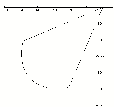
Figure 3.3‑c

Moreover, with this choice of coefficients, some simple compression traction paths had snap-backs as indicated in the appendix.

We then preferred to replace condition number 4 of [Tableau 3.3-a] by a condition expressing that, after the traction limit had returned to zero, the reversibility domain is that represented on [Figure 3.3-d].

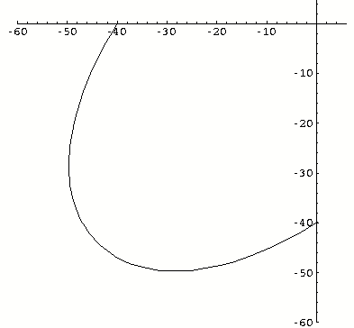
Figure 3.3‑d

This leads to the replacement of the \(c+3\alpha d=\sqrt{2}\) relationship by \(c=\sqrt{2}\)

The choice of the coefficients a, b, c and d is finally:

\(a=\sqrt{2}\frac{\beta -1}{2\beta -1}b=\frac{\sqrt{2}}{3}\frac{\beta }{2\beta -1}\) eq 3.3‑ 3.3-3

\(c=\sqrt{2}d=\frac{2\sqrt{2}}{3}\) eq 3.3‑ 3.3-4

Figure 3.3‑e

The [Figure 3.3-e] shows the difference between the two models for a plane stress state.

3.4. Analysis of the selected reversibility domain

In this chapter, we give indications on the order of magnitude of the admissible stresses in the sense of the criterion adopted. We focus on providing information on tensile stresses, in particular for three-dimensional stress states.

[Figure 3.4-a] shows the initial domains (i.e. before work hardening) for the following values of the material parameters:

\({f}_{c}^{\text{'}}\)	initial rupture limit in simple compression:	\({f}_{c}^{\text{'}}\) = 40 Mpa
\({f}_{\text{cc}}^{\text{'}}\)	initial break limit in bi compression	\({f}_{\text{cc}}^{\text{'}}\) =44 Mpa
\(\beta =\frac{{f}_{\text{cc}}^{\text{'}}}{{f}_{c}^{\text{'}}}\)	ratio between rupture limit in bi-compression and simple compression	:math:`beta ` = 1.1
\(\phi {f}_{c}^{\text{'}}\)	elastic limit in compression;	\(\varphi =\mathrm{0,33}\)
\({f}_{t}^{\text{'}}\)	initial tensile failure limit	\({f}_{t}^{\text{'}}\) = 4 Mpa

Figure 3.4‑a

Figures [Figure 3.4-b], [Figure 3.4-c] and [Figure 3.4-d] show the sections of the three-dimensional domain by planes \({\sigma }_{3}=0\) and \({\sigma }_{3}=-25\text{Mpa}\)

Figure 3.4‑b

Figure 3.4‑c

Figure 3.4‑d

The [Figure 3.4-e] shows the reversibility domains in a \(({\sigma }_{1},{\sigma }_{2})\) plane for constant \({\sigma }_{3}\) stress states, domains parameterized by the value of \({\sigma }_{3}\). We represent the domains for \({\sigma }_{3}=-25\text{Mpa}\), \({\sigma }_{3}=0\text{Mpa}\), \({\sigma }_{3}=4\text{Mpa}\),,, \({\sigma }_{3}=10\text{Mpa}\), \({\sigma }_{3}=15\text{Mpa}\). It can be seen that for a confinement of 25 Mpa of compression, the tensile stresses can reach \(15\mathit{Mpa}\), and that, at the same time, the reversibility domain for \({\sigma }_{3}=15\text{Mpa}\) is not empty and corresponds to compression stresses \({\sigma }_{1}\) and \({\sigma }_{2}\) of order of \(\mathrm{-}25\mathit{Mpa}\). We also see that, for a given value of \({\sigma }_{3}\), the maximum traction value

Obtained for \({\sigma }_{1}\) and \({\sigma }_{2}\) is achieved at the intersection of traction and compression criteria.

Figure 3.4‑e

We are therefore studying where the traction and compression criteria intersect. We note \(({\sigma }_{H}^{0},{\sigma }_{0}^{\text{eq}})\) the intersection point of the two criteria in plane \(({\sigma }_{H},{\sigma }^{\text{eq}})\) (point C of the [Figure 3.4-f]).

Figure 3.4‑f

The place of intersection of the two criteria in the constraint space is given by:

\(\{\begin{array}{}{\sigma }_{1}=\frac{2}{3}{\sigma }_{0}^{\text{eq}}\mathrm{sin}(\theta +\frac{\pi }{6})+{\sigma }_{H}^{0}\\ {\sigma }_{2}=\frac{2}{3}{\sigma }_{0}^{\text{eq}}\mathrm{sin}(-\theta +\frac{\pi }{6})+{\sigma }_{H}^{0}\\ {\sigma }_{3}=3{\sigma }_{H}^{0}-{\sigma }_{1}-{\sigma }_{2}\end{array}\)

Where \(\theta\) is a parameter.

Figure 3.4‑g

The [Figure 3.4-g] shows the projections of this place in plans \(({\sigma }_{\mathrm{1,}}{\sigma }_{2})\) and \(({\sigma }_{\mathrm{2,}}{\sigma }_{3})\).

We can easily calculate the maximum stress value along this curve:

\({\sigma }_{\mathrm{max}}=\frac{{f}_{c}^{\text{'}}}{3}+\frac{2}{3\beta }{f}_{t}^{\text{'}}\) eq 3.4‑ 3.4-1

This equation shows that, regardless of the value chosen for the tensile failure limit, the maximum tensile stress reached is greater than a third of the compressive failure limit.

[Figure 3.4-h] shows the three main constraints as a function of the \(\theta\) parameter.

Figure 3.4‑h

We can see that we can reach a traction level of \(15\mathit{Mpa}\), but for a lockdown of \({\sigma }_{2}=-25\text{Mpa}\) and \({\sigma }_{3}=-25\text{Mpa}\).

To try to avoid this drawback, which is important, we can try to play on the values of the compression resistance and the parameter :math:`beta `.

As an example, we chose the following set of parameters:

\({f}_{c}^{\text{'}}\mathrm{=}20\mathit{Mpa}\)

\({f}_{\text{cc}}^{\text{'}}\mathrm{=}40\mathit{Mpa}\)

\(\beta \mathrm{=}2\)

\({f}_{t}^{\text{'}}\mathrm{=}4\mathit{Mpa}\)

The [Figure 3.4-i] shows the criteria with this choice of parameters. The [Figure 3.4-j] shows the value of the main constraints at the intersection of the two criteria for this new choice of parameters. The maximum traction obtained is lower (\(8\mathit{Mpa}\)), but it is achieved for a lower level of confinement (\(\mathrm{-}\mathrm{7Mpa}\)).

Figure 3.4‑i

Figure 3.4‑j

3.5. Work hardening

As already mentioned in paragraph [§ 3.3], when the stress state reaches the edge of the reversibility domain, plastic deformations and internal variables develop, the thresholds shift: they collapse. For our model, the internal variables are two in number, they are noted \({\kappa }_{c}^{p}\) for the internal variable « called compression » and \({\kappa }_{t}^{p}\) for the internal variable « called tension ». These variables determine the evolution of the compression and traction thresholds respectively; the thermodynamic forces are linked to them by the relationships:

\({A}_{c}=\phi {f}_{c}^{\text{'}}-{f}_{c}({\kappa }_{c}^{p})\) eq 3.5‑ 3.5-1

and

\({A}_{t}={f}_{t}^{\text{'}}-{f}_{t}({\mathrm{\kappa }}_{t}^{p})\) eq 3.5‑ 3.5-2

where \({f}_{c}({\mathrm{\kappa }}_{c}^{p})\) and \({f}_{t}({\mathrm{\kappa }}_{t}^{p})\) represent the values of the compressive and tensile resistances respectively.

3.5.1. Work hardening functions

The function \({f}_{c}({\mathrm{\kappa }}_{c}^{p})\) is first increasing then decreasing, the decreasing part being either linear [Figure 3.5.1-a], or quadratic [Figure 3.5.1-b],

Figure 3.5.1-a

Figure 3.5.1-b

\(\phi\) is model data. The shape of the curve between \({\mathrm{\kappa }}_{c}^{e}\) and \({\mathrm{\kappa }}_{c}^{e}\) (negative work hardening) depends on the element, and more precisely on its dimensions, according to a criterion similar to that chosen by G.Heinfling, [Error: Reference source not found] to take into account the location of the deformations.

In traction, the shape of the curve giving the value of the elastic limit \({f}_{t}({\kappa }_{t}^{p})\) as a function of the cumulative plastic deformation \({\mathrm{\kappa }}_{t}^{p}\) does not include a « pre-peak » part, the « post-peak » part being either linear [Figure 3.5.1-c] or exponential [Figure 3.5.1-d].

Figure 3.5.1-c

Figure 3.5.1-d

3.5.2. Work hardening curves and post peak modules

3.5.2.1. Distributed cracking pattern

The introduction of post-peak softening behavior into stress-strain relationships poses a major problem. Under static stress, beyond a certain level of stress, corresponding to the onset of softening behavior, the equations governing the balance of the structure lose their elliptical nature. These equations of the mechanical problem then form a system of poorly posed partial differential equations whose number of solutions is multiple. This problem results in non-objectivity in relation to the mesh. This results in a pathological sensitivity of the numerical solution to the fineness and orientation of the mesh.

In order to solve this problem, or at least to limit its consequences on the reliability of the predicted solution, it is necessary to use so-called regularization techniques. The purpose of these techniques is to enrich the mechanical description of the environment, in order to be able to describe non-homogeneous states of deformation, and to preserve the mathematical nature of the problem. This regularization is carried out by introducing, into the law of behavior, a characteristic length or internal length, linked to the width of the location zone. Several techniques are possible to improve the mechanical description of the softening medium. They are location limiters. The implementation of these techniques generally requires delicate digital developments. An intermediate approach between the use of classical models and the implementation of these location limiters consists in making the post-peak slope depend on the stress-strain relationship, on the size of the element, so as to dissipate constant energy at break. This approach is a step towards a non-local description of the continuous environment.

Let us first consider a real crack on surface \(S\) whose measurement is A [Figure 3.5.2.1-a]. \(S\) is a discontinuous surface of the \(u\) displacement field. It is assumed that to create this discontinuity, it is necessary to expend an energy \(W\) whose expression is: \(\text{W=}{\int }_{S}{G}_{f}(x)\text{dS}\), \({G}_{f}\) being a property of the material.

Let us now consider that we want to represent the same phenomenon, by representing not a discontinuity of displacement but a plastic deformation uniformly distributed in a volume \(V\).

The energy dissipated will be: \(\text{W=}{\int }_{v}\text{dV}{\int }_{0}^{{t}_{r}}{\sigma }^{\mathrm{ij}}\frac{d{\mathrm{\varepsilon }}_{\mathrm{ij}}^{p}}{\mathrm{dt}}\mathrm{dt}\), where we noted

the « breakup time. »

Figure 3.5.2.1-a

By making the following series of hypotheses:

• the crack is flat,

• \({G}_{f}\) is constant along the crack and therefore \(\text{W=}A\text{.}{G}_{f}\),

• \(V\) is a cylinder with a base \(S\) and a height of \({L}_{\text{ver}}\),

• \({g}_{f=}{\int }_{0}^{{t}_{t}}{\mathrm{\sigma }}^{\text{ij}}\frac{{\mathrm{d\varepsilon }}_{\text{ij}}^{p}}{\text{dt}}\text{dt}\) is constant in \(V\).

We finally end up with the relationship:

\(W={\text{Vg}}_{f}=V{\int }_{0}^{{t}_{t}}{\mathrm{\sigma }}^{\text{ij}}\frac{{\mathrm{d\varepsilon }}_{\text{ij}}^{p}}{\text{dt}}\text{dt}=A\text{.}{G}_{f}\) eq 3.5.2.1-1

Or even:

\({g}^{f}={\int }_{0}^{{t}_{r}}{\sigma }^{\mathrm{ij}}\frac{d{\mathrm{\varepsilon }}_{\mathrm{ij}}^{p}}{\mathrm{dt}}\mathrm{dt}=\frac{{G}_{f}}{{L}_{\mathrm{ver}}}\) eq 3.5.2.1-2

We can easily see that: \({g}^{f}={\int }_{0}^{{\mathrm{\kappa }}_{u}}f(\mathrm{\kappa })\mathrm{d\kappa }\), writing in which the quantities \(({g}^{f},f,{\mathrm{\kappa }}_{u},\mathrm{\kappa })\) represent respectively \(({g}_{t}^{f},{f}_{t},{\mathrm{\kappa }}_{t}^{u},{\mathrm{\kappa }}_{t}^{p})\) in tension and \(({g}_{c}^{f},{f}_{c},{\mathrm{\kappa }}_{c}^{u},{\mathrm{\kappa }}_{c}^{p})\) in compression. The data of \({g}^{f}\) therefore determines \({k}_{u}\), this in tension as well as in compression:

\({g}_{c}^{f}={\int }_{0}^{{k}_{c}^{u}}f({\mathrm{\kappa }}_{c}^{p}){\mathrm{d\kappa }}_{c}^{p}=\frac{{G}_{c}^{f}}{{L}_{\mathrm{ver}}}\)

\({g}_{t}^{f}={\int }_{0}^{{k}_{t}^{u}}f({\mathrm{\kappa }}_{t}^{p}){\mathrm{d\kappa }}_{t}^{p}=\frac{{G}_{t}^{f}}{{L}_{\mathrm{ver}}}\)

Quantity \({g}^{f}\) is therefore linked to the slope of the post-peak curve in a stress-variable work hardening diagram, which is linked to the post-peak slope in a stress-strain diagram.

For example, suppose that the stress-strain relationship is linear in post-peak conditions. Let’s call \({E}_{T}<0\) the post-peak slope in diagram \((\sigma ,\varepsilon )\) and \(h<0\) the corresponding slope in diagram \((f,\mathrm{\kappa })\) [Figure 3.5.2.1-b]. We have the \(h=\frac{{\text{EE}}_{T}}{E-{E}_{T}}\iff {E}_{T}=\frac{\text{hE}}{E+h}\) relationships that show that we need to have:

\(-h<E\), otherwise diagram \((\sigma ,\varepsilon )\) shows a snap back.

Figure 3.5.2.1-b

Condition \(-h<E\) is called the applicability condition, it will result in an inequality on \({g}^{f}\) and therefore on \({L}_{\text{ver}}\).

In the context of a resolution by the finite element method, the elementary volume representative of the cracked medium can be assimilated to an element of the mesh. The characteristic length (subsequently noted \({l}_{c}\)) introduced in the equivalent breaking energy method corresponds to the length \(\mathit{Lver}\). During a calculation corresponding to any structure, the determination of this characteristic length is difficult. It depends on the position of the crack plane, the dimensions and the type of the elements…

A simple estimate for two-dimensional cases can be expressed in the form:

\({l}_{c}=r\sqrt{{A}_{e}}\) where \({A}_{e}\) is the area of the element in question, and \(r\), a correction factor, equal to 1 for quadratic elements, and \(\sqrt{2}\) for linear elements.

We can extend this formulation to the 3D case: \({l}_{c}=r\sqrt[3]{{V}_{e}}\) where \({V}_{e}\) refers to the volume of the element.

Regarding the evolution of work hardening with temperature, we consider as in [bib2] that the rupture energies and the rupture resistances do not depend on the current temperature

from the material point considered at time \(t\), but from the maximum temperature reached at this point from the start of loading to time \(t\). When we need to show the dependence of quantities on temperature, we will note:

• \(\theta\) the maximum temperature since the start of loading,

• \({f}_{c}^{\text{'}}(\theta )\) the compressive strength,

• \({f}_{t}^{\text{'}}(\theta )\) refers to tensile strength,

• \({f}_{c}(\theta ,{\mathrm{\kappa }}_{c}^{p})\) the compressive work hardening curve,

• \({f}_{t}(\theta ,{\mathrm{\kappa }}_{t}^{p})\) the tensile work hardening curve.

3.5.2.2. Tensile behavior of concrete and linear post-peak curve

In this modeling, concrete is assumed to be elastic up to its tensile strength \({f}_{t}^{\text{'}}\). Tensile curve \({f}_{t}({\mathrm{\kappa }}_{t}^{p})\) is shown on [Figure 3.5.1-c] and is entirely defined by the tensile strength of the material, the crack energy \({G}_{t}^{f}\), and the characteristic length \({l}_{c}\).

The mathematical expression for this curve is:

\({f}_{t}(\mathrm{\theta },{\mathrm{\kappa }}_{t}^{p})={f}_{t}^{\text{'}}(\mathrm{\theta })(1-\frac{{\mathrm{\kappa }}_{t}^{p}}{{\mathrm{\kappa }}_{t}^{u}(\mathrm{\theta })})\) eq 3.5.2.2-1

The equivalence of the energy dissipated makes it possible to write:

\({G}_{t}^{f}(\theta )={l}_{c}\underset{0}{\overset{{\kappa }_{t}^{u}}{\int }}{f}_{t}(\theta ,{\kappa }_{t}^{p})={l}_{c}{f}_{t}^{\prime }(\theta )\underset{0}{\overset{{\kappa }_{t}^{u}}{\int }}(1-\frac{{\kappa }_{t}^{p}}{{\kappa }_{t}^{u}(\theta )})d{\kappa }_{t}^{p}\)

whence

\({G}_{t}^{f}(\mathrm{\theta })=\frac{{l}_{c}\text{.}{f}_{t}^{\prime }(\mathrm{\theta })\text{.}{\mathrm{\kappa }}_{t}^{u}(\mathrm{\theta })}{2}\) eq 3.5.2.2-2

and

\({\mathrm{\kappa }}_{t}^{u}(\mathrm{\theta })=\frac{2\text{.}{G}_{t}^{f}(\mathrm{\theta })}{{l}_{c}\text{.}{f}_{t}^{\prime }(\mathrm{\theta })}\) eq 3.5.2.2-3

The condition of applicability is written as:

\({l}_{c}\le \frac{2\text{.}E(\mathrm{\theta })\text{.}{G}_{t}^{f}(\mathrm{\theta })}{{f}_{t}^{{\prime }^{2}}(\mathrm{\theta })}\) eq 3.5.2.2-4

3.5.2.3. Tensile behavior of concrete and post-peak exponential curve

In this modeling, concrete is assumed to be elastic up to its tensile strength

. Tensile curve \({f}_{t}({\kappa }_{t}^{p})\) is shown on [Figure 3.5.1-d] and is entirely defined by the tensile strength of the material, the crack energy \({G}_{t}^{f}\), and the characteristic length \({l}_{c}\).

The mathematical expression for this curve is:

\({f}_{t}(\mathrm{\theta },{\mathrm{\kappa }}_{t}^{p})={f}_{t}^{\text{'}}(\mathrm{\theta })\text{.}\text{exp}(-a\frac{{\mathrm{\kappa }}_{t}^{p}}{{\mathrm{\kappa }}_{t}^{u}(\mathrm{\theta })})\) eq 3.5.2.3-1

The equivalence of the energy dissipated makes it possible to write:

\({G}_{t}^{f}(\mathrm{\theta })={l}_{c}\underset{0}{\overset{\infty }{\int }}{f}_{t}(\mathrm{\theta },{\mathrm{\kappa }}_{t}^{p})={l}_{c}{f}_{{t}^{\prime }}(\mathrm{\theta })\underset{0}{\overset{\infty }{\int }}\text{exp}(-a\frac{{\mathrm{\kappa }}_{t}^{p}}{{\mathrm{\kappa }}_{t}^{u}(\mathrm{\theta })}){\mathrm{d\kappa }}_{t}^{p}\)

From where:

\({G}_{t}^{f}(\mathrm{\theta })=\frac{{l}_{c}\text{.}{f}_{t}^{\prime }(\mathrm{\theta })\text{.}{\mathrm{\kappa }}_{t}^{u}(\mathrm{\theta })}{a}\) eq 3.5.2.3-2

and

\(\frac{{\mathrm{\kappa }}_{t}^{u}(\mathrm{\theta })}{a}=\frac{{G}_{t}^{f}(\mathrm{\theta })}{{l}_{c}\text{.}{f}_{t}^{\prime }(\mathrm{\theta })}\) eq 3.5.2.3-3

Let’s say again: \({f}_{t}(\mathrm{\theta },{\mathrm{\kappa }}_{t}^{p})={f}_{t}^{\text{'}}(\mathrm{\theta })\text{.}\text{exp}(-{l}_{c}\text{.}{f}_{t}^{\text{'}}(\mathrm{\theta })\frac{{\mathrm{\kappa }}_{t}^{p}}{{G}_{t}^{f}(\mathrm{\theta })})\)

The maximum slope of the curve is then \({h}_{\text{max}}(\mathrm{\theta })=\frac{-{l}_{c}\text{.}{f}_{t}^{{\prime }^{2}}(\mathrm{\theta })}{{G}_{t}^{f}(\mathrm{\theta })}\)

and the condition of applicability is written as:

\(\begin{array}{cc}{l}_{c}\le \frac{E(\mathrm{\theta })\text{.}{G}_{t}^{f}(\mathrm{\theta })}{{f}_{t}^{{\prime }^{2}}(\mathrm{\theta })}& \forall \mathrm{\theta }\end{array}\) eq 3.5.2.3-4

3.5.2.4. Compression behavior of concrete and linear post-peak curve

In this modeling, the behavior of concrete is assumed to be elastic up to the elastic limit, given by a proportionality coefficient (noted \(\phi\) as a percentage of peak strength \({f}_{c}^{\text{'}}(\theta )\)). For standard concrete \(\phi\) is in the order of 30%. The compression curve \({f}_{c}({\kappa }_{c}^{p})\) is shown on [Figure 3.5.1-a] and is entirely defined by the tensile strength of the material, the crack energy \({G}_{c}^{f}\), and the characteristic length \({l}_{c}\).

The mathematical expression for this curve is:

\(\{\begin{array}{cccc}{f}_{c}(\theta ,{\kappa }_{c}^{p})=f{\text{'}}_{c}(\theta )(\phi +(2-2\varphi )\frac{{\kappa }_{c}^{u}}{{\kappa }_{e}(\theta )}+(\phi -1)\frac{{\kappa }_{c}^{{p}^{2}}}{{\kappa }_{{e}^{2}}(\theta )})& \text{si}& {\kappa }_{c}^{p}\le {\kappa }_{e}(\theta )& \text{éq}3\text{.}5\text{.}2\text{.}4-1\\ {f}_{c}(\theta ,{\kappa }_{c})=f{\text{'}}_{c}(\theta )(\frac{({\kappa }_{c}^{p}-{\kappa }_{c}^{u}(\theta ))}{({\kappa }_{e}(\theta )-{\kappa }_{c}^{u}(\theta ))})& \text{si}& {\kappa }_{e}(\theta )\le {\kappa }_{c}^{p}\le {\kappa }_{c}^{u}(\theta )& \text{éq}3\text{.}5\text{.}2\text{.}4-2\end{array}\)

Maximum compressive strength is reached when: \({\kappa }_{e}(\theta )=(2-2\phi )\frac{{f}_{c}^{\prime }(\theta )}{E(\theta )}\)

The equivalence of the energy dissipated makes it possible to write:

\({G}_{c}^{f}(\theta )={l}_{c}\underset{0}{\overset{{\kappa }_{c}^{u}}{\int }}{f}_{c}(\theta ,{\kappa }_{c}^{p})d{\kappa }_{c}^{p}\)

whence

\({G}_{c}^{f}(\theta )={l}_{c}\text{.}{f}_{c}^{\prime }(\theta )(\frac{2\phi +1}{6}{\kappa }_{e}(\theta )+\frac{1}{2}{\kappa }_{c}^{u}(\theta ))\) eq 3.5.2.4-3

and

\({\kappa }_{c}^{u}(\theta )=\frac{2\text{.}{G}_{c}^{f}(\theta )}{{l}_{c}\text{.}{f}_{c}^{\prime }(\theta )}-\frac{2\phi +1}{3}{\kappa }_{e}(\theta )\) eq 3.5.2.4-4

The slope of the curve is then \(h(\mathrm{\theta })=-\frac{{f}_{c}^{\prime }(\mathrm{\theta })}{{\mathrm{\kappa }}_{c}^{u}(\mathrm{\theta })-{\mathrm{\kappa }}_{e}(\mathrm{\theta })}\)

and the condition of applicability is written as:

\(\begin{array}{cc}{l}_{c}\le \frac{E(\theta )\text{.}{G}_{c}^{f}(\theta )}{{f}_{c}^{{\prime }^{2}}(\theta )}\frac{6}{\text{11}-4\phi -4{\phi }^{2}}& \forall \theta \end{array}\) eq 3.5.2.4-5

3.5.2.5. Compression behavior of concrete and non-linear post-peak curve

In this modeling, the behavior of concrete is assumed to be elastic up to the elastic limit, given by a proportionality coefficient (noted \(\phi\) as a percentage of peak strength). \({f}_{c}^{\text{'}}(\theta )\). For standard concrete \(\phi\) is in the order of 30%. The compression curve \({f}_{c}({\kappa }_{c}^{p})\) is shown on [Figure 3.5.1-b] and is entirely defined by the tensile strength of the material, the crack energy \({G}_{c}^{f}\), and the characteristic length \({l}_{c}\).

The mathematical expression for this curve is:

\(\{\begin{array}{cccc}{f}_{c}(\theta ,{\kappa }_{c}^{p})={f}_{c}^{\text{'}}(\theta )(\phi +(2-2\phi )\frac{{\kappa }_{c}^{p}}{{\kappa }_{e}(\theta )}+(\phi -1)\frac{{\kappa }_{c}^{{p}^{2}}}{{\kappa }_{{e}^{2}}(\theta )})& \text{si}& {\kappa }_{c}^{p}\le {\kappa }_{e}(\theta )& \text{éq}3\text{.}5\text{.}2\text{.}5-1\\ {f}_{c}(\theta ,{\kappa }_{c})={f}_{c}^{\text{'}}(\theta )(1-\frac{{({\kappa }_{c}^{p}-{\kappa }_{e}(\theta ))}^{2}}{{({\kappa }_{c}^{u}(\theta )-{\kappa }_{e}(\theta ))}^{2}})& \text{si}& {\kappa }_{e}(\theta )\le {\kappa }_{c}^{p}\le {\kappa }_{c}^{u}(\theta )& \text{éq}3\text{.}5\text{.}2\text{.}5-2\end{array}\)

Maximum compressive strength is reached when: \({\kappa }_{e}(\theta )=(2-2\phi )\frac{{f}_{c}^{\prime }(\theta )}{E(\theta )}\)

The equivalence of the energy dissipated makes it possible to write:

\({G}_{c}^{f}(\mathrm{\theta })={l}_{c}\underset{0}{\overset{{\mathrm{\kappa }}_{c}^{u}}{\int }}{f}_{c}(\mathrm{\theta },{\mathrm{\kappa }}_{c}^{p}){\mathrm{d\kappa }}_{c}^{p}\)

from where:

\({G}_{c}^{f}(\theta )={l}_{c}\text{.}{f}_{c}^{\prime }(\theta )(\frac{2}{3}{\kappa }_{c}^{u}(\theta )+\frac{\phi }{3}{\kappa }_{e}(\theta ))\) eq 3.5.2.5-3

and:

\({\kappa }_{c}^{u}(\theta )=\frac{3}{2}\frac{{G}_{c}^{f}(\theta )}{{l}_{c}\text{.}{f}_{c}^{\prime }(\theta )}-\frac{\phi }{2}{\kappa }_{e}(\theta )\) eq 3.5.2.5-4

The maximum slope of the post-peak curve is then \({h}_{\text{max}}(\mathrm{\theta })=-\frac{2\text{.}{f}_{c}^{\prime }(\mathrm{\theta })}{{\mathrm{\kappa }}_{c}^{u}(\mathrm{\theta })-{\mathrm{\kappa }}_{e}(\mathrm{\theta })}\)

and the condition of applicability is written as:

\(\begin{array}{cc}{l}_{c}\le \frac{3}{2}\frac{E(\theta )\text{.}{G}_{c}^{f}(\theta )}{{f}_{c}^{{\prime }^{2}}(\theta )}\frac{1}{4-\phi -{\phi }^{2}}& \forall \theta \end{array}\) eq 3.5.2.5-5