8. example

It is [Figure 6-a] the plane pendulum movement of an extendable bar \(\mathrm{AB}\) of unit length, rotated in \(A\) to a fixed support, free in \(B\) and abandoned without speed in the Earth’s gravity field from a position defined by the angle \({\theta }_{0}\). All mechanical dissipation phenomena are overlooked.

As the amplitude \({\theta }_{0}\) can be large — we will take it from \(90°\) — the point \(B\) undergoes large displacements and the problem is non-linear.

The theoretical period is:

\(T=\mathrm{1,6744}s\)

The calculation of the pendulum movement using diagram HHT (\(\alpha\) -method) with \(\alpha =0\) (« trapezium rule ») constitutes test case SDNL100.

Figure [Figure 6-b] represents the evolution over a period of time in the dimension of point \(B\) calculated by the « modified mean acceleration » scheme with three values of \(\alpha\). The period is divided into 40 equal time steps.

The solid line curve is relative to \(\alpha =0\). Practically no errors are observed.

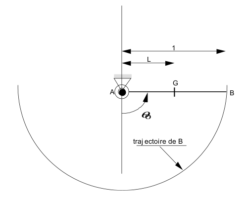
Figure 6-a: Large amplitude pendulum

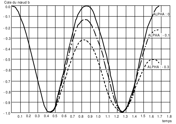
Figure 6-b: « Modified mean acceleration » diagram, 40 steps of 0.0419 s

The centreline curve is relative to \(\alpha =-\mathrm{0,1}\). We observe a depreciation rate of around 2% while figure [Figure 6-a], for \(\frac{\mathrm{\Delta }t}{T}=\mathrm{0,025}\), forecasts 0.8%. This is because this curve was established linearly, while the movement of our pendulum is non-linear.

The dashed curve is relative to \(\alpha =-\mathrm{0,3}\). The depreciation rate is around 5.8%, while that predicted by figure [Figure 5.3-a] is around 2.2%. The discrepancy is still due to the non-linearity of the problem.

Finally, the centreline and especially dashed curves reveal a shortening of the calculated period compared to the theoretical period.