2. The second expansion gradient model

The principle of microstructure media is based on taking into account microscopic deformations in order to introduce an internal length into the expression of the model. While the effectiveness of the regularization provided by the second gradient model is beyond doubt, simulation calculation times can become prohibitive. To reduce them in the particular context of dilating materials (for which the volume deformation changes as a function of loading), the generality of the regularizing effect is restricted to dilating microstructure media.

2.1. Expanding microstructure media

The kinematics of these media are defined by the usual field of displacement \({u}_{i}\), the microscopic volume variation noted \(\chi\) and its gradients. By duality to this enriched kinematics, the static variables of classical macroscopic constraints \({\sigma }_{\text{ij}}\), the microscopic expansion stress \(\kappa\) and the double vector expansion constraints \({S}_{j}\) are introduced. The variable \(\kappa\) is the conjugate component of the relative volume deformation (of the macroscopic field compared to the microscopic field) \({\epsilon }_{V}-\chi\), while the components \({S}_{j}\) define a vector that is the conjugate of the microscopic expansion gradient \(\frac{\partial \chi }{\partial {x}_{j}}\).

Analogous to the expression of the virtual power of microstructure media in chapter 1.1, and again neglecting the expression of external volume forces for analytical simplification, we find \(({u}_{i}^{\text{*}},{\chi }^{\text{*}})\) for dilating microstructure media, for any kinematically admissible field

(2.1)\[ \ underset {\ omega} {\ int} ({\ sigma}} _ {\ text {ij}}}\ frac {\ partial {u} _ {i} ^ {\ text {*}}}} {\ partial {x}} _ {j}}} +\ kappa ({\ epsilon}}} +\ kappa ({\ epsilon}} _ {V}} ^ {\ text {*}}} - {\ chi} ^ {\ chi} ^ {\ text {x} _ {j}}}} {\ partial {x} _ {j}}} +\ kappa ({\ epsilon}} _ {j}}} +\ kappa ({\ epsilon}} _ {j}}}}) + {S} _ {j}\ frac {\ partial {\ chi} ^ {\ text {*}}} {\ partial {x} _ {j}})\ text {dv} =\ underset {\ partial\ Omega} {\ omega} {\ omega} {\ omega} {\ omega} {\ omega} {\ omega}} {\ int} {\ int}} {\ int}} ({t} _ {i}} {u} _ {i}} ^ {\ text {*}}} =\ underset {\ partial\ Omega}} {\ partial\ Omega} {\ omega} {\ omega}} {\ int} {\ int}} ({t} _ {i}} {u} _ {i}} ^ {\ text {*}}} =\ underset {\ partial\ chi}} ^ {\ text {*}}})\ text {ds}\]

For which

(2.2)\[ {t} _ {i} =\ left ({\ sigma}} _ {\ text {ij}} _ {\ text {ij}}} _ {\ text {ij}}\ right) {n} _ {j}\]

(2.3)\[ m= {S} _ {j} {n} {n} _ {j}\]

are the boundary conditions, expressed on border \(\partial \mathrm{\Omega }\), conjugated by duality to the kinematic variables \({u}_{i}\) and \(\chi\) respectively.

The equilibrium relationships for this problem are written

(2.4)\[ \ frac {\ partial {\ sigma} _ {\ text {ij}}}} {\ partial {x} _ {j}} +\ frac {\ partial\ kappa} {\ partial\ kappa} {\ partial {x}} _ {i}} =0\]

(2.5)\[ \ kappa +\ frac {\ partial {S} _ {j}} {\ partial {x} _ {j}} =0\]

The system of equations composed of [(), (), (), () and ()] is obtained classically by applying the divergence theorem and by integrating by part of ().

2.2. The second expansion gradient model

According to a principle similar to that implemented for the second gradient model in chapter 1.2, a mathematical constraint is introduced to force equality between macroscopic \({\epsilon }_{V}\) and microscopic \(\chi\) volume deformations.

(2.6)\[ \ chi = {\ epsilon} _ {V}\]

The expression for virtual powers is then as follows, for any kinematically admissible field \({u}_{i}^{}\)

(2.7)\[ \ underset {\ omega} {\ int} ({\ sigma}} _ {\ text {ij}}}\ frac {\ partial {u} _ {i} ^ {\ text {*}}}} {\ partial {x} _ {j}} _ {j}}} + {S}}} + {S}}} + {S}}} + {S}}} + {S} _ {j}}} {\ partial {x} _ {i}\ partial {x} _ {j}}})\ text {dv}} =\ underset {\ partial\ Omega} {\ int} ({p} _ {i} {u} _ {u} _ {i} _ {i} _ {i} _ {i} _ {i}} _ {i} _ {i} _ {i} _ {i} _ {u} _ {u} _ {u} _ {u} _ {u} _ {u} _ {u} _ {u} _ {u} _ {u} _ {i} _ {u} _ {u} _ {u} _ {i} _ {u} _ {u} _ {u} _ {i} _ {u} _ {u} _ {u} _ {i} _ {u}}})\ text {ds}\]

where \({p}_{i}\) and \(P\) are the boundary conditions defined by

(2.8)\[ {p} _ {i} = {\ sigma} _ {\ text {ij}} _ {j}} {n} - {n} _ {i} {n} _ {\ text {DS}} _ {j}} _ {j} -\ frac {\ text {j}} -\ frac {{\ text {ij}}} _ {j}} {n}} _ {j}} _ {j}} _ {j}} _ {j}} _ {j}} _ {j}} _ {j}} _ {j}} _ {j}} _ {j}} _ {j}} _ {j}} _ {i}} - {i} - {i} - {i} - {frac {\ text {DS}} _ {j} {n} _ {n} _ {j}}} {{\ text {Dx}}} _ {i}} +\ frac {{\ text {Dn}} _ {p}}} {{\ text {Dx}}} {{j}}} {n}} _ {n}} _ {n} _ {i}} {i}\]

(2.9)\[ P= {S} _ {j} {n} {n} _ {j}\]

As for the second gradient model, the hypothesis on the equality between microscopic and macroscopic volume deformation fields () has a direct impact on the expression of boundary conditions because the variables \({u}_{i}^{\text{*}}\) and \({\chi }^{\text{*}}\) are no longer independent.

For the sake of simplicity, we assume \(P=0\). The consequence of this assumption is that \({S}_{j}{n}_{j}=0\) on the border, which reduces the expression () to

(2.10)\[ {p} _ {i} = {\ sigma} _ {\ text {ij}} {\ text {ij}}} {n} -\ frac {\ partial {S} _ {j}}} {\ partial {x}} _ {x} _ {x} _ {x} _ {x} _ {x} _ {x} _ {x} _ {x} _ {x} _ {x} _ {x} _ {x} _ {x} _ {j}}\]

A remarkable property of this simplification comes from the fact that the expression of boundary conditions is then broken down into the classical part \({\sigma }_{\text{ij}}{n}_{j}\) and a second term that does not induce shear components.

The equilibrium equation is written as:

\[\]

: label: eq-20

frac {partial {sigma} _ {text {ij}}}} {partial {j}}} {partial {x}}} -frac {{partial} ^ {2} {S} _ {j}} _ {j}}} {partial {j}}}} {partial {x}}} =0

2.3. Spatial discretization by finite elements

2.3.1. Historical discretization of the second expansion gradient model

The aim of the second dilation gradient approach is to define a regularizing model, making it possible to ensure the independence of the results with respect to spatial discretizations, by introducing a minimum of nodal unknowns into its finite element approach. For this purpose, we are limited to applications involving dilating materials. However, discretizing the expression () by the finite element method has the consequence of requiring that the field of displacement unknowns as well as its divergence be continuous and differentiable. This is equivalent to taking into account C1-continuous finite elements.

It is then proposed to introduce the mathematical constraint () into the expression of dilating microstructure media by means of a coupling of Lagrange and penalization multipliers. We then obtain for any kinematically admissible field \(\left({u}_{i}^{\text{*}},{\chi }^{\text{*}},{\lambda }^{\text{*}}\right)\)

\[\]

: label: eq-21

begin {array} {c}underset {mathrm {omega}} {mathrm {omega}}} {int}left ({sigma} _ {i}}frac {partial {u} _ {i}} ^ {i} ^ {i} ^ {i} ^ {i} ^ {i} ^ {i} ^ {i} ^ {i} ^ {i} ^ {text {*}}}}} {partial {*}}}} {int}left ({sigma}} _ {ij}}}frac {partial {chi}} ^ {chi}} ^ {chi}}} {partial {*}}}} {partial {*}}}} {partial {*}}}} {partial {text {*}}} {partial {x} _ {j}}} -lambdaleft ({epsilon} _ {V} ^ {text {*}}} - {chi} ^ {text {*}} _ {text {*}}right) + {text {*}}right) + {lambda}}right) + {lambda}} ^ {text {*}}}left ({epsilon} _ {V}} - {V} -chiright) +rleft ({epsilon} _ {V} -chiright)left ({epsilon} _ {V} ^ {text {*}}} - {chi} ^ {text {*}}\ right}}right)right)right)right)text {dv}right)right)text {*}}right)right)right)right)text {dv}right)right)right)right)text {dv}right)right)right)right)text {dv}}\ phantom {rule {2em} {0ex}}text {=}text {*}}text {*}}text {*}}text {*}}partialmathrm {Omega}} {int}} {int}left ({p}left ({p}} _ {i} _ {i}} ^ {text {*}}} + {text {Pn}}} _ {text {Pn}}} _ {text {i}}} + {text {Pn}}} _ {text {Pn}}} _ {i}} _ {text {Pn}}} _ {i}} _ {text {Pn}}} _ {i}}} {*}}right)text {ds}end {array}

this historical formulation is available under the name DIL. The proposed digital implementation is detailed in chapter 3. Here only the approximation spaces of the variables defining the kinematic field are specified. The polynomial interpolations are P2-P1-P1 (in plane deformations and in 3D):

1. second order shape functions for displacement variables \(u\)

2. first-order shape functions for the microscopic volume strain tensor \(\chi\) and the Lagrange multipliers \(\lambda\)

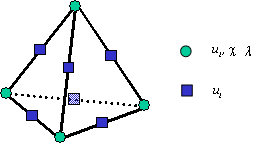
Figure 2.3-a: Finite element discretization of the second expansion gradient model for 3D.

2.3.2. Incompressible modeling of the second expansion gradient model

This modeling proposed by Gantier [14] is a variation of the modeling presented in the paragraph adapted to behaviors where dilation tends to zero with work hardening. This modeling is based on incompressible elements with three fields (see R3.06.08). It is not available for THM models with a second gradient.

(2.11)\[\begin{split} \ begin {array} {c}\ underset {\ mathrm {\ Omega}} {\ mathrm {\ omega}}} {\ int}\ left ({\ mathrm {}}} _ {\ mathit {ij}}} _ {\ mathit {ij}}}}} ^ {D}} ^ {D} (u\ text {*}}) +\ frac {1} {3}\ chi\ text {}}} _ {\ mathit {ij}}} _ {\ mathit {ij}}} _ {\ mathit {ij}}}} ^ {D} (u\ text {*}}) +\ frac {1} {3}\ chi\ text {thrm {\ delta}} _ {\ mathit {ij}}}\ right) + {S} _ {j}\ frac {\ partial {\ chi} ^ {\ text {*}}} {\ partial {x} _ {j}}} +\ mathit {ij}}}\ right) +\ mathit {ij}}} +\ mathit {ij}}} +\ mathit {ij}}} +\ mathit {ij}}} +\ mathit {ij}}} +\ lambda\ j}}} +\ lambda\ left ({\ epsilon} _ {j}}} +\ lambda\ left ({\ epsilon} _ {j}}} +\ lambda\ left ({\ epsilon}} _ {\ text {*}}}} {\ chi} *}}\ right) + {\ lambda} ^ {\ text {*}}}\ left ({\ epsilon} _ {V} -\ chi\ right) +r\ left ({\ epsilon} _ {V} _ {V} -\ chi\ right)\\ chi\ right)\ left ({\ epsilon}} _ {V}} ^ {\ text {*}}} - {\ chi} _ {V}}} - {\ chi} _ {V}} - {\ chi} ^ {\ chi} ^ {\ text {*}} ^ {\ chi} ^ {\ text {*}}}}\ right)\ right)\ text {dv}\\\ phantom {\ rule {2em} {0ex}}\ text {=}\ underset {\ partial\ mathrm {\ mathrm {\ Omega}}} {\ omega}}} {\ int}\ left ({p} _ {i} {u} _ {i} ^ {\ text {*}}} + {\ text {*}}} + {\ text {Pn}} _ {i}} ^ {\ text {*}}}\ right)\ text {*}}\ right)\ text {ds}\ end {array}\end{split}\]

In this expression, \({\mathrm{ϵ}}^{D}\) represents deviatoric deformation and \({\mathrm{\delta }}_{\mathit{ij}}\) represents the Kronecker symbol.

This formulation is therefore inspired by incompressible elements with three fields: it is the variable \(\chi\) that intervenes in the law of first gradient behavior.

Moreover, it has been shown (see Gantier [14]) that the use of the term penalization is optional: the use of a Lagrange multiplier is sufficient to impose equality between microscopic and macroscopic volume deformations.

The shape functions used are identical to those of the historical formulation of the second gradient. They are of the P2-P1-P1 type:

1. second order shape functions for displacement variables \(u\)

2. first-order shape functions for the microscopic volume strain tensor \(\chi\) and the Lagrange multipliers \(\lambda\)