4. Implementation in Code_Aster#
The behavior relationship ASSE_CORN is assigned to discrete modeling elements DIS_TR with 2 nodes combined. This relationship is called by the nonlinear problem solving operators STAT_NON_LINE [R5.03.01] or DYNA_NON_LINE [R5.05.05].
The local axes of these x, y, z elements are defined as on [Figure 2-a].
Integrating this relationship of assembly behavior into the operator STAT_NON_LINE of Code_Aster requires the formulation of the tangent operators \({K}_{o}\) and \({K}_{n}\) [bib3].
\({K}_{o}\) is the tangent stiffness at the start of the time step, instant \(t\).
\({K}_{n}\) is the tangent stiffness at the end of the time step, instant \(\text{t+dt}\).
The illustration of the operators \({K}_{o}\) and \({K}_{n}\) is given by the [Figure 4-a].
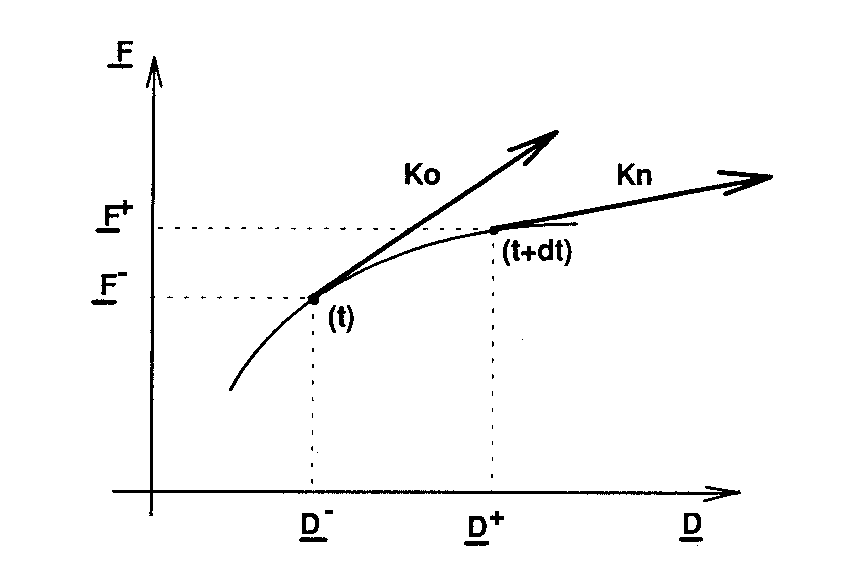
Figure 4-a: definition of operators \({K}_{o}\) and \({K}_{n}\)
4.1. Formulation in reduced quantities during loading#
4.1.1. Operator \({K}_{\mathit{nr}}\)#
We saw in [§3.2] that the behavioral relationship is written as:
\(\begin{array}{c}\begin{array}{}{\underline{f}}^{\text{+}}=\frac{\mathrm{\Delta }\underline{d}}{\mathrm{\Delta \; p}}R({p}^{\text{-}}+\mathrm{\Delta \; p})\\ \text{avec}\mathrm{\Delta \; p}=\parallel \mathrm{\Delta }\underline{d}\text{.}\mathrm{\Delta }\underline{d}\parallel =\sqrt{{\mathrm{\Delta \; U}}_{r}^{2}+{\mathrm{\Delta \; \theta }}_{r}^{2}}\end{array}\end{array}\)
The \({K}_{\text{nr}}\) operator is defined by:
\(\begin{array}{c}{K}_{\text{nr}}=\left[\frac{\partial {f}_{i}}{\partial {d}_{j}}\right]1\le i,j\le 2\end{array}\)
It is written:
\(\begin{array}{}{K}_{\text{nr}}=\frac{\mathrm{\Delta \; p}\left[\text{Id}\right]-\left\{\mathrm{\Delta }\underline{d}\right\}\text{.}<\frac{\partial \mathrm{\Delta \; p}}{\partial {\mathrm{\Delta \; d}}_{j}}{>}^{\text{+}}}{{\mathrm{\Delta \; p}}^{2}}R({p}^{\text{+}})+\left\{\mathrm{\Delta }\underline{d}\right\}\text{.}<\frac{\partial \mathrm{\Delta \; p}}{\partial {\mathrm{\Delta \; d}}_{j}}{>}^{\text{+}}\frac{R\text{'}({p}^{\text{+}})}{\mathrm{\Delta \; p}}\\ \end{array}\)
The calculation then gives:
\(\begin{array}{}\text{<}\frac{\partial \mathrm{\Delta \; p}}{\partial {\mathrm{\Delta \; d}}_{j}}{>}^{\text{+}}\text{=}(\frac{{\mathrm{\Delta \; U}}_{r}}{\mathrm{\Delta \; p}};\frac{{\mathrm{\Delta \; \theta }}_{r}}{\mathrm{\Delta \; p}})\\ \left\{\mathrm{\Delta }\underline{d}\right\}\text{.}<\frac{\partial \mathrm{\Delta \; p}}{\partial {\mathrm{\Delta \; d}}_{j}}{>}^{\text{+}}\text{=}\left[\begin{array}{cc}\frac{{\mathrm{\Delta \; U}}_{r}^{2}}{\mathrm{\Delta \; p}}& \frac{{\mathrm{\Delta \; U}}_{r}{\mathrm{\Delta \; \theta }}_{r}}{\mathrm{\Delta \; p}}\\ \frac{{\mathrm{\Delta \; U}}_{r}{\mathrm{\Delta \; \theta }}_{r}}{\mathrm{\Delta \; p}}& \frac{{\mathrm{\Delta \; \theta }}_{r}^{2}}{\mathrm{\Delta \; p}}\end{array}\right]\end{array}\)
and with \(\underline{a\mathrm{=}1}\) (the only case currently being treated), we have: \(h(x)\mathrm{=}\frac{1}{\overline{d}}\frac{{x}^{2}}{1\mathrm{-}x}\)
\(\begin{array}{}R(p)={h}^{\text{- 1}}(p)=\frac{1}{2}(-\overline{d}p+\sqrt{{\overline{d}}^{2}{p}^{2}+4\overline{d}p})\\ R\text{'}(p)=\frac{1}{h\text{'}\left[R(p)\right]}=\frac{\overline{d}{\left[1-R(p)\right]}^{2}}{R(p)\left[2-R(p)\right]}\end{array}\)
4.1.2. Operator \({K}_{\text{or}}\)#
For elasto-plastic behaviors, the operator \({K}_{o}\) to \(t\mathrm{=}0\) is equal to the stiffness of the elastic structure. In our case, the initial tangent behavior is rigid. The operator \({K}_{\text{or}}\) is then defined by the passage to the limit when \(p\) tends to 0 of the operator \({K}_{\text{nr}}\). We get:
\(\begin{array}{}R\text{'}(p)\underset{p\to 0}{\text{=}}\frac{R(p)}{p}\\ \text{d'où}{K}_{\text{or}}\underset{p\to 0}{\text{=}}\frac{R(p)}{p}\left[\text{Id}\right]\end{array}\)
Now \(R(p)<1\forall p\) and if we assume that the user gives, for the first loading step, values such as \(\mathrm{\Delta \; p}>{\text{10}}^{\text{-}4}\), we can remember in practice:
\({K}_{{\text{or}}_{t=0}}=\left[\begin{array}{cc}{\text{10}}^{4}& 0\\ 0& {\text{10}}^{4}\end{array}\right]\)
This value by default can be modified (see §5).
These words are illustrated by the [Figure 4.1.2-a].
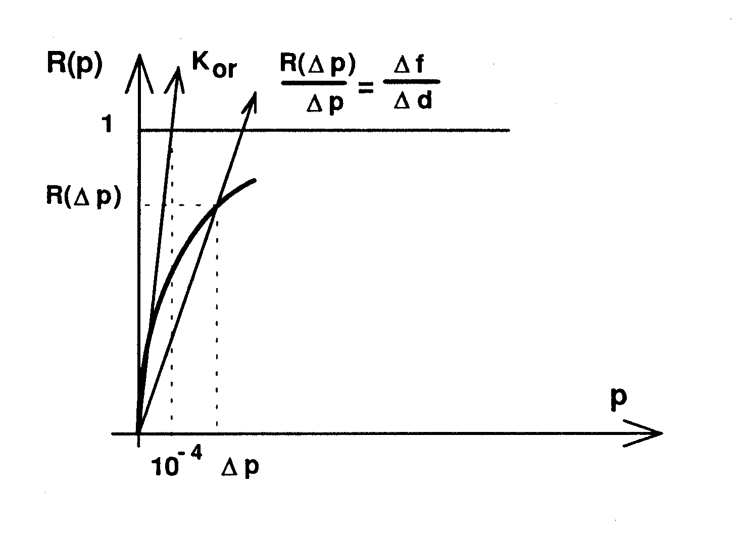
Figure 4.1.2-a: Ko operator at t = 0
At the current moment \(t\), the \({K}_{\text{or}}\) operator is equal to the \({K}_{\text{nr}}\) operator of the previous step defined by the [§4.1.1].
4.2. Formulation in reduced quantities when unloaded#
To avoid numerical problems, the (rigid) unloading behavior is described by:
\(\begin{array}{c}{K}_{\text{or}}={K}_{\text{nr}}={K}_{{\text{or}}_{t=0}}\end{array}\)
4.3. Tangent operators \({K}_{n}\) and \({K}_{o}\)#
The tangent operator \({K}_{n}\) is written, based on the reduced tangent operator calculated in §4.1.
\(\begin{array}{c}{K}_{n}=\left[\frac{\partial {F}_{i}}{\partial {D}_{j}}\right]1\le i,j\le 6\end{array}\)
with
\(\begin{array}{}\frac{\partial {F}_{1}}{\partial {D}_{1}}=\frac{\partial {N}_{x}}{\partial U}=\frac{\partial n}{\partial {U}_{r}}\times \frac{\overline{N}}{\overline{U}}\\ \frac{\partial {F}_{1}}{\partial {D}_{5}}=\frac{\partial {N}_{x}}{\partial \mathrm{\theta }}=\frac{\partial n}{\partial {\mathrm{\theta }}_{r}}\times \frac{\overline{N}}{\overline{\mathrm{\theta }}}\\ \frac{\partial {F}_{5}}{\partial {D}_{1}}=\frac{\partial {M}_{y}}{\partial U}=\frac{\partial m}{\partial {U}_{r}}\times \frac{\overline{M}}{\overline{U}}\\ \frac{\partial {F}_{5}}{\partial {D}_{5}}=\frac{\partial {M}_{y}}{\partial \mathrm{\theta }}=\frac{\partial m}{\partial {\mathrm{\theta }}_{r}}\times \frac{\overline{M}}{\overline{\mathrm{\theta }}}\\ \frac{\partial {F}_{2}}{\partial {D}_{2}}={K}_{y}\\ \frac{\partial {F}_{3}}{\partial {D}_{3}}={K}_{z}\\ \frac{\partial {F}_{4}}{\partial {D}_{4}}={\text{KR}}_{x}\\ \frac{\partial {F}_{6}}{\partial {D}_{6}}={\text{KR}}_{z}\end{array}\)
Other values are zero.
The tangent operator \({K}_{o}\), at \(t\) = 0, is written as:
\({K}_{o}=\left[\begin{array}{cccccc}{\text{10}}^{4}\frac{\overline{N}}{\overline{U}}& & & & O& \\ & {K}_{y}& & & & \\ & & {K}_{z}& & & \\ & & & {K}_{\text{Rx}}& & \\ O& & & & {\text{10}}^{4}\frac{\overline{M}}{\overline{\mathrm{\theta }}}& \\ & & & & & {K}_{\text{Rz}}\end{array}\right]\)
4.4. Numerical treatment of the connection between the mechanisms of the law of assembly#
During the resolution of each of the loading steps by Newton’s iterative method, the tangent to the force-displacement balance curve of the law of behavior must be calculated at each iteration. The problem is that the connection between the mechanisms of the law of assembly, on the law of behavior, has a positive concavity (cf. [Figure 2-b]) which makes convergence problematic when, during a loading step, one passes from one mechanism to the other.
In subroutine TE0041, which calculates, for each load increment, the elementary tangential stiffness matrix of a discrete finite element with 2 knots possessing degrees of freedom in translation and rotation, it proved necessary to converge, to calculate a secant stiffness directed from the initial state of zero effort and displacement to the state, at the end of the loading step, constituted by the imposed force and the corresponding displacement on the Equilibrium curve of the law of behavior. To do this, which was unusual for this option, it was necessary to know the internal iteration number of the numerical process calculating the loading step, and then to estimate the effort imposed on the element at the end of this step.
In fact, if we note \({F}^{\text{+}}\) the effort imposed at the level of an element (a priory unknown since we only know the combined forces), \({U}^{\text{+}}\) the corresponding displacement on the balance curve, and for iteration \(i\), the respective values \(U(i),F(i),Ks(i)\) of the displacement, the effort and the secant matrix — acting as a tangent matrix — calculated at the end of the iteration, we only know at the input of the aforementioned subroutine \({U}^{i}\), and the values at the start of the load step \(F(0)\) and \(U(0)\), because we didn’t store the values at the previous iteration \(i\mathrm{-}1\). In the expression for the residue calculated at the end of iteration \(i\mathrm{-}1\): \({F}^{\text{+}}-F(i-1)={K}_{s}(i-1)\text{.}(U(i)-U(i-1))\), we therefore only know \(U(i)\) at iteration \(i\), except in the particular case \(i\mathrm{=}1\) where we have:
\({F}^{\text{+}}-F(0)={K}_{s}(0)\text{.}(U(1)-U(0))\)
\({F}^{+}\) y is the only value unknown at the start and can be inferred from the others. We also deduce the displacement \({U}^{\text{+}}\) at the end of the step according to the equilibrium relationship:
\(\stackrel{\text{.}}{p}\text{.}\left[n,m\right]=R(p)\text{.}\left[{\stackrel{\text{.}}{U}}_{r},{\stackrel{\text{.}}{\mathrm{\Theta }}}_{r}\right]\), hence the secant stiffness \({K}_{s}(1)={F}^{\text{+}}/{U}^{\text{+}}\).
The problem is that in this first iteration, the imposed displacement \(U(1)\) is different from the final displacement to be calculated \({U}^{\text{+}}\) in balance with \({F}^{+}\) now known (in the balance test near the previous loading step). The effort calculated at the end of this iteration \(F(1)\) must therefore also be different from \({F}^{+}\) and such as \(F(1)={K}_{s}(1)\text{.}U(1)\) so that starting from the pair \(U(1)\) and \(F(1)\), we point with the secant \({K}_{s}(1)\) to the pair \({U}^{\text{+}}\) and \({F}^{\text{+}}\). At the start of iteration 2, we thus obtain a displacement \(U(2)\) that is very close to \({U}^{\text{+}}\) and we can then calculate by the equilibrium relationship \(F(2)\), which is also very close to \({F}^{\text{+}}\), as well as the secant stiffness \({K}_{s}(2)=F(2)/U(2)\).
If we have converged exactly at the previous load step, 2 internal iterations are sufficient to converge exactly, otherwise a few additional iterations are needed to satisfy the balance test on the residue.
The so-called « directed secant » method is schematized on [Figure 4.3-a] where we have the following matches:
\(\begin{array}{}{U}^{i}=U(i)\\ {K}_{t}({U}^{i})={K}_{s}(i)\end{array}\)
for a \(\text{LC}({U}^{i})=F(i)\) law of behavior.

Figure 4.3-a: directed secant method
We therefore now see why it was necessary to know the internal iteration number \(i\) in the option calculated by the abovementioned subroutine in order to distinguish the particular case \(i\mathrm{=}1\).
Variables and parameters of the law of behavior
4.5. Variables of the law#
The law of behavior includes 7 internal variables per calculation point:
\(\mathit{V1}\) is the maximum equivalent reduced displacement p achieved in mechanism 1,
\(\mathit{V2}\) is the maximum reduced displacement equivalent p achieved in mechanism 2,
\(\mathit{V3}\) is an indicator that is equal to 1 or 2 depending on whether one is respectively on the limit surface of mechanism 1 or 2, and 0 if one is under this limit surface (after discharge for example),
\(\mathit{V4}\) and \(\mathit{V5}\) are respectively the maximum force and moment reached in mechanism 2 before discharge,
\(\mathit{V6}\) and \(\mathit{V7}\) are respectively the original displacement and rotation of mechanism 1, which can be non-zero when after unloading in mechanism 2, the loading changes sign to return to mechanism 1.
4.6. parameters of the law#
The parameters of the law of behavior are entered as data under the ASSE_CORN keyword from the DEFI_MATERIAU [U4.43.01] command:
NU_1: behind this keyword we enter the value of the parameter \({\overline{N}}_{1}\) of the mechanism 1,
MU_1: behind this keyword we enter the value of the parameter \({\overline{M}}_{1}\) of the mechanism 1,
DXU_1: behind this keyword we enter the value of the parameter \({\overline{U}}_{1}\) of the mechanism 1,
DRYU_1: behind this keyword we enter the value of the parameter \({\overline{\mathrm{\theta }}}_{1}\) of the mechanism 1,
C_1: behind this keyword we enter the value common to the parameters \(\stackrel{ˉ}{n}\) and \(\stackrel{ˉ}{m}\) of the mechanism 1,
NU_2: behind this keyword we enter the value of the parameter \({\overline{N}}_{2}\) of the mechanism 2,
MU_2: behind this keyword we enter the value of the parameter \({\overline{M}}_{2}\) of the mechanism 2,
DXU_2: behind this keyword we enter the value of the parameter \({\overline{U}}_{2}\) of the mechanism 2,
DRYU_2: behind this keyword we enter the value of the parameter \({\overline{\mathrm{\theta }}}_{2}\) of the mechanism 2,
C_2: behind this keyword we enter the value common to the parameters \(\stackrel{ˉ}{n}\) and \(\stackrel{ˉ}{m}\) of the mechanism 2,
KY, KZ, KRX, KRZ take the values of the linear behavior characteristics in the local directions « * respectively,
RP_0: a possible value of \({K}_{\text{or}}\) (104 by default) is entered behind this keyword.
Note :: ** Parameter \(a\) is not accessible to the user. It is set to the value \(a\mathrm{=}1\).