2. Continuous model

All the equations of the model are combined in the table. The link between the internal parameters of the model and the quantities more accessible to the engineer is also specified. The modeling choices call for a few remarks, which are set out below.

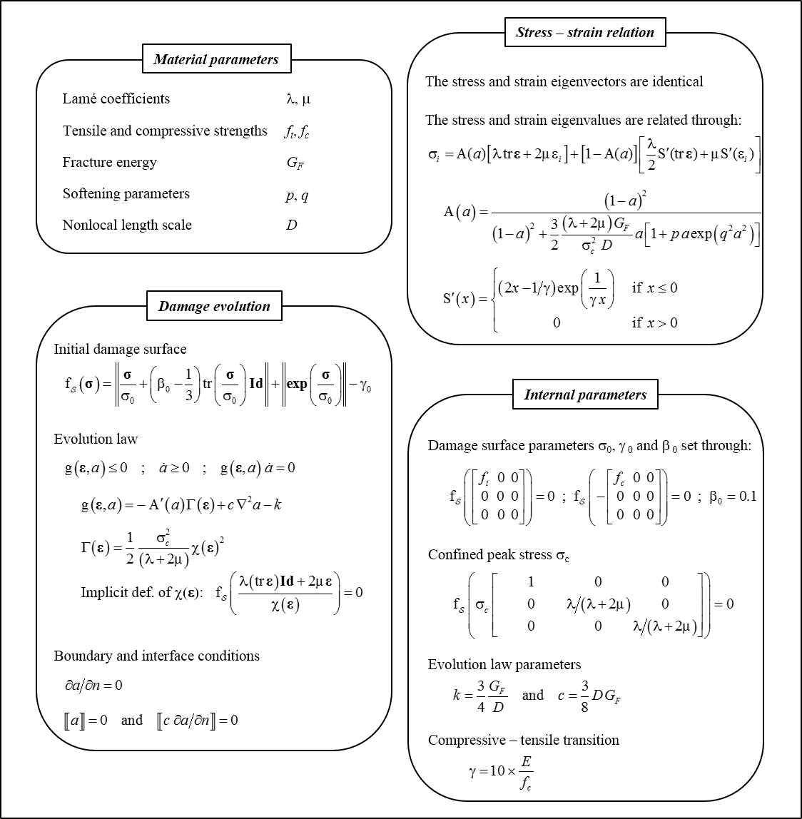
Table 2-1: Continuous Model Equations

2.1. Stress-deformations relationship

Function \(A(a)\), which is involved in the stress-deformation relationship, measures the impact of the level of damage on residual stiffness (under tension). Its particular form is guided by consistency with a cohesive law. It plays the same role as the more classical form in (1- a) used in a number of models in the literature.

Moreover, to take into account the restoration of stiffness under compression, the law of elasticity is no longer linear, even if it remains hyperelastic (i.e. it derives from energy) in order to avoid any parasitic production or consumption of energy. It is similar to the formulation adopted for law ENDO_ISOT_BETON [R7.01.04]; it takes into account not only the sign of the deformations itself but also that of the trace of the deformations. In practice, it therefore requires determining the eigenvalues of the deformation tensor.

Finally, to improve the robustness of the model and the convergence of the calculation, the stiffness jump during the tensile — compression transition was regularized, using the infinitely differentiable \(S(x)\) function. It ensures a gradual transition between a zero value and a quadratic function; the speed (or brutality) of the transition is controlled by the parameter \(\gamma\). A value by default is proposed in the DEFI_MATER_GC command, which states that 90% of the stiffness without regularization is found for a deformation (in compression) of the order of \(\mathit{fc}/E\).

2.2. Evolution of damage

The presence of a damage term in Laplacian in the threshold function as well as a boundary condition on the damage field of zero normal gradient at the edge reflects the non-local nature of the model. More precisely, this corresponds to the non-local formulation with an internal variable gradient as introduced in the fascicle [R5.04.01]. On the numerical level, it allows an (almost) classical treatment of the law of behavior. However, the choice of a phenomenologically acceptable damage surface leads to the renunciation of the existence of a single functional energy to describe all the equations of the problem. Here, the evolution of the damage and the balance of the structure result from the minimization of two distinct functional energies. In practice, the tangent operator is then no longer symmetric.