Shock and friction modeling DIS_CONTACT#
Behavior DIS_CONTACT reflects contact with shock and friction between two structures, via two types of relationships:
the unilateral contact relationship which expresses the non-inter-penetrability between solid bodies,
the friction relationship that governs the variation of tangential forces in contact. For the present developments, a simple relationship will be retained: Coulomb’s law of friction.
- lookout
This behavior is integrated with a direct implicit time schema and is written as a classical law of behavior. The stiffness and damping parameters that are involved in this behavior are therefore « physical ».
- Recommendation
In the case where the stiffness is no longer « physical » but rather « penalizing », it is desirable to use behavior DIS_CHOC, which has the same material parameters and whose relationship is integrated explicitly by treating contact and friction by penalization.
Unilateral contact relationship#
Defining distances for relationship DIS_CHOC.#
Definition of contact distance#
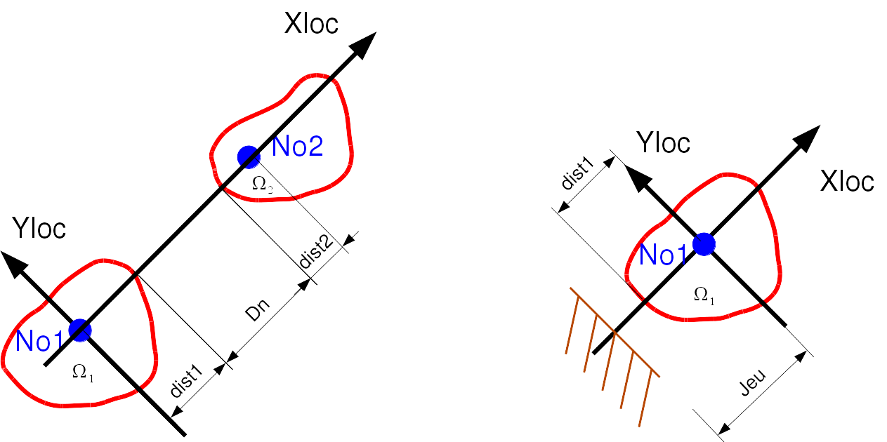
We define the contact distance \(d_c\). In the case of a discrete with 2 knots of length \(l_d\)
In the case of a discrete with 1 node:
The contact distance is positive in the direction of the local axis \({X}_{\text{loc}}\). To establish initial contact, it is therefore necessary to choose the values of the parameters wisely. \(\dist_1\), \(\dist_2\), and \(\text{jeu}\)
Formulation of behavior#
The formulation of the behavior is very similar to that found in perfect plasticity.
Friction is represented by a threshold describing nonlinear behavior.
The elastic stiffness along the local axes \({K}_{x},{K}_{y},{K}_{z}\).
Under these conditions:
Where:
\({F}_{cy}\) and \({F}_{cz}\): Coulomb’s tangent efforts..
\({F}_{x}\): normal effort.
\({\mu}\): Coulomb coefficient of friction.
The behavior is described by the following equations:
The efforts in the discreet are:
If \(f\le 0\):
If \(f=0\) and \(\dot{f}=0\):
with
and
Coulomb friction is governed by behavior equations () and (). An example of a loading path is shown in Figure r5.03.17-fig-EvolutionFrottementCoulomb.
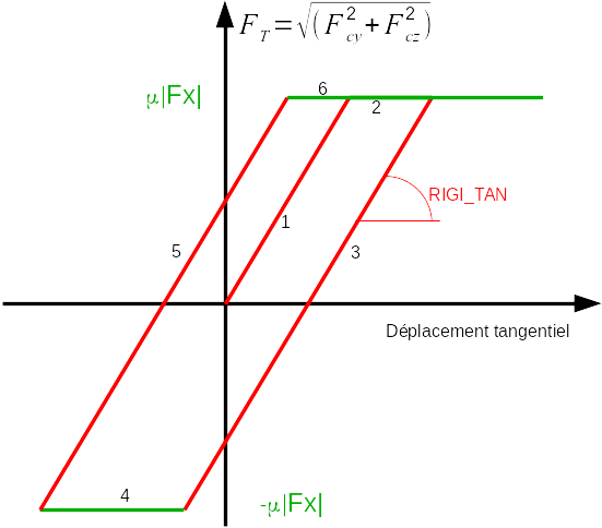
Evolution of Coulomb friction.#
The loading path is as follows:
loading with stiffness RIGI_TAN up to the Coulomb threshold.
sliding on the threshold.
unloading with stiffness RIGI_TAN up to the threshold.
sliding on the threshold.
charging up to the threshold.
sliding on the threshold.
Local integration of behavior#
The scheme used is that of Runge-Kutta of order 5 with error control. Figure RK5 is a combination of the 4th order diagram and the 6th order diagram [bib9], for which the coefficients are determined so as to minimize the error between order 4 and order 6.
The local integration of this model uses the 5th order RUNGE - KUTTA schema.
The error between orders 4 and 5 is known, so it is possible to trigger local subdivisions of the time step if the convergence criterion is not met.
Defining contact parameters#
Here are the keywords used to define the parameters of contact, damping and friction in DEFI_MATERIAU [U4.43.01]:
The RIGI_NOR operand allows you to give the value of the normal shock stiffness \({K}_{N}\).
The AMOR_NOR operand allows you to give the value of the normal shock absorption \({C}_{N}\).
The RIGI_TAN operand allows you to give the value of the tangential stiffness \({K}_{T}\).
The AMOR_TAN operand allows you to give the value of the tangential shock damping \({C}_{T}\).
The COULOMB operand is used to give the value of the Coulomb coefficient.
The DIST_1 operand defines the characteristic distance of matter surrounding the first shock node
The DIST_2 operand defines the characteristic distance of material surrounding the second shock node (shock between two mobile structures).
The operand JEU defines the distance between the shock node and an unmodelled obstacle (case of a shock between a mobile structure and an undeformable and immobile obstacle).
Operand EVOLJEU which is a function of the multiplicative time of JEU. This function makes it possible to progressively establish the contact distance, as defined above.
Internal variables#
There are nine of them:
\(V1\): component of the tangent force along the local axis \(y\): \({F}_{cy}\).
\(V2\): component of the tangent force along the local axis \(z\): \({F}_{cz}\).
\(V3\): displacement due to sliding in the tangential plane along the local \(y\) axis.
\(V4\): displacement due to sliding in the tangential plane along the local \(z\) axis.
\(V5\): speed along the local \(x\) axis.
\(V6\): speed along the local \(y\) axis.
\(V7\): speed along the local \(z\) axis.
\(V8\): management of the initial interpenetration of the discrete.
\(V9\): initial contact management.