Shock and friction modeling DIS_CHOC

Behaviour DIS_CHOC reflects contact with shock and friction between two structures, via two types of relationships:

• the unilateral contact relationship which expresses the non-inter-penetrability between solid bodies,

• the friction relationship that governs the variation of tangential forces in contact. For the present developments, a simple relationship will be retained: Coulomb’s law of friction.

lookout

This behavior is explicit and is treated by penalization. The stiffness that occurs in behavior is therefore not « physical ». It is not recommended to use this behavior to model elements whose stiffness has a « physical » meaning.

Recommendation

It is desirable and recommended, in the case where stiffness has a physical meaning, to use behavior DIS_CONTACT, which has the same material parameters and with a formalism similar to a law of plasticity.

Unilateral contact relationship, in the discrete frame of reference

Defining distances for relationship DIS_CHOC

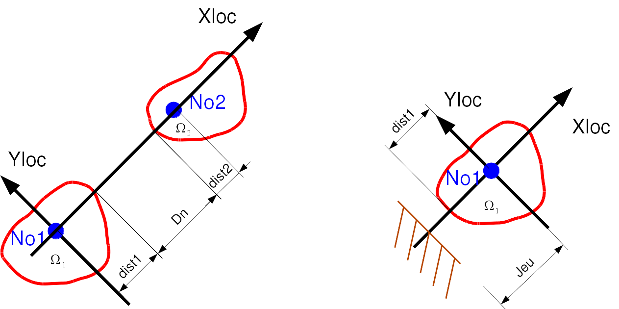
• In the case of a discrete with 2 knots (based on a SEG2).

  Let’s say two structures \({\Omega}_{1}\) and \({\Omega}_{2}\). Note \({d}_{N}\) the normal distance between structures, \({F}_{N}^{1/2}\) the normal reaction force of \({\Omega}_{1}\) over \({\Omega}_{2}\).

  In the coordinate system local to the element, there will be « shock » when \({d}_{N}\le 0\). The expression for the normal distance \({d}_{N}\) is:

  \[\DeclareMathOperator{\dist}{dist} {d}_{N} = (({X}_{\text{loc}2}^{0}+{u}_{2})-({X}_{\text{loc}1}^{0}+{u}_{1}))-{\dist}_{1}-{\dist}_{2}\]

• In the case of a discrete to one node (based on a POI1).

  There is only one \({\Omega}_{1}\) structure. Note \({d}_{N}\) the normal distance between the structure and the shock plane (which is not modelled). \({F}_{N}^{1/2}\) the normal reaction force of \({\Omega}_{1}\) on the plane.

  In the coordinate system local to the element, the normal distance \({d}_{N}\) is expressed as:

  \[{d}_{N} = {u}_{1}+(\text{jeu}-{\dist}_{1})\]

  There will be « shock » when \({d}_{N}\le 0\).

The law of action and reaction imposes

\[{F}_{N}^{2/1} = -{F}_{N}^{1/2}\]

The conditions of unilateral contact, also called Signorin [bib5] conditions, are expressed in the following way:

\[\begin{split}\left \{ \begin{array}{ll} {d}_{N}\ge 0 \\ {F}_{N}^{1/2}\ge 0 \\ {d}_{N} \, {F}_{N}^{1/2}=0 \end{array} \right. \text{ et } {F}_{N}^{2/1}=-{F}_{N}^{1/2}\end{split}\]

Graph of the one-sided contact relationship.

Graph r5.03.17-fig-Signorini reflects a force-displacement relationship that is not differentiable. It is therefore not easy to use in a dynamic calculation algorithm.

Unilateral contact relationship, in the global frame of reference of the mesh

In this case the discrete is 2 knots (based on a SEG2).

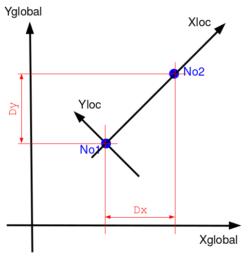
Definition of distances for relationship DIS_CHOC, in the global coordinate system

We note:math: dist the distance between the 2 nodes:math:`dist=left ({D} _ {x}, {D} _ {y}right) `. The contact is effective when the 2 distances are negative. The contact effort is calculated in the global coordinate system: math: `F_ {x|y} = K,minleft (vert {D} _ {x}green,vert {D} _ {d} _ {y}vertright) `.

The principle of penalization, presented in Normal contact force model, applies in the same way.

notes

The behavior of the discrete is treated in the global coordinate system, so it must be in one of the planes \(XY\), \(XZ\) or \(YZ\). If this is not the case an error is issued. Compared to the case of the shock discrete treated in the local coordinate system, here the parameters \(\dist_{1}\) and \(\dist_{2}\) no longer have physical meaning, they are therefore not taken into account. An error is issued in the case of an inconsistency in the parameters.

Coulomb’s law of friction

Coulomb’s law expresses a limitation of the tangential force \({F}_{T}^{1/2}\) of tangential reaction of \({\Omega}_{1}\) on \({\Omega}_{2}\). Let \({\dot{u}}_{T}^{1/2}\) be the relative speed of \({\Omega}_{1}\) with respect to \({\Omega}_{2}\) at a point of contact and let \(\mu\) be the Coulomb coefficient of friction, we have [bib5].

\[s = \Vert {F}_{T}^{1/2} \Vert - \mu \, {F}_{N}^{1/2} \le 0 \quad \exists \lambda {\dot{u}_{T}^{1/2}} = \lambda {F}_{T}^{1/2} \lambda \le 0 \lambda s = 0\]

and the law of action and reaction:

\[{F}_{T}^{2/1} = -{F}_{T}^{1/2}\]

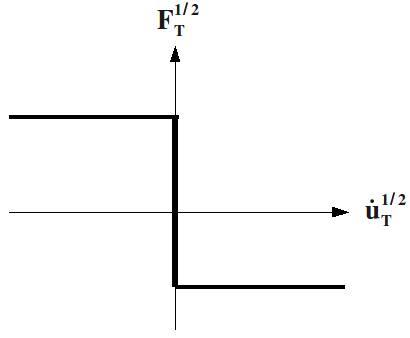
Graph of Coulomb’s law of friction.

Graph r5.03.17-fig-Coulomb of Coulomb’s law is also non-differentiable and is therefore not easy to use in a dynamic algorithm.

Approximate modeling of contact relationships by penalization

Normal contact force model

The principle of penalization consists in introducing an unequivocal \({F}_{N}^{1/2}={f}_{{\epsilon}}\left({d}_{N}\right)\) relationship by means of a parameter \(\varepsilon\). The \({f}_{\varepsilon}\) graph should tend towards the Signorin graph when \(\varepsilon\) tends to zero [bib6].

One of the possibilities is to propose a linear relationship between \({d}_{N}\) and \({F}_{N}^{1/2}\):

\[\begin{split}\begin{cases} \text{Si} & {d}_{N}\le 0 & \text{ alors } &{F}_{N}=\frac{1}{\epsilon}{d}_{N} \\ \text{Sinon} & {F}_{N}=0 > 0 \end{cases}\end{split}\]

If we note \({K}_{N} = \frac{1}{\varepsilon}\), commonly called shock stiffness, we find the classical relationship, modeling an elastic shock:

\[{F}_{N}^{1/2} = -{K}_{N} \, {d}_{N}^{1/2}\]

Approximate graph r5.03.17-fig-ContactPenalisation of the law of contact with penalization is as follows:

Graph of the unilateral contact relationship approximated by penalization

In dynamics, to take into account a possible loss of energy in the shock, we introduce « shock absorption » \({C}_{N}\). The expression for the normal contact force is then expressed as:

()\[{F}_{{N}^{1/2}} = - {K}_{N}\, {d}_{N}-{C}_{N}\, {\dot{u}}_{{N}^{1/2}}\]

where \({\dot{u}}_{N}^{1/2}\) is the relative normal speed of \({\Omega}_{1}\) compared to \({\Omega}_{2}\). To respect the Signorin relationship (no adherence in contact), \({F}_{N}^{1/2}\) must be positive or zero. So we will only take the positive part \({\langle \rangle }^{+}\) of the expression ():

\[\begin{split}\left \{ \begin{array}{ll} {\langle x\rangle }^{\text{+}}=x & \text{si } x\ge 0 \\ {\langle x\rangle }^{+}=0 & \text{si } x < 0 \end{array} \right.\end{split}\]

The complete relationship giving the normal contact force that is retained for the algorithm is as follows

()\[\begin{split}\left. \begin{array}{l} \text{Si} & d_N \le 0 & F_N^{1/2}={⟨-K_N \, d_N-C_N \, {\dot{u}}_N^{1/2}⟩}^{\text{+}} & F_N^{2/1}=-F_N^{1/2} \\ \text{Sinon} & F_N^{2/1}=F_N^{1/2}=0 \end{array} \right\}\end{split}\]

note

This model of contact by penalty involves a normal penalty stiffness \(K_N\) and a damping \(C_N\). The objective of this modeling is to have no interpenetration by involving a force that will oppose interpenetration.

• During a static calculation, this effort is given by () with \(\dot{u}=0\).

• During a dynamic calculation, the effort is always given by (). When treating contact by penalization, stiffness (here \(K_N\)) is chosen. by the user to limit interpenetration. So there is no reason for this stiffness to have a physical sense. This stiffness, which is often great compared to the stiffness of the other elements, intervenes on the diagonal of the assembled matrix of the problem. During a calculation dynamic, it is possible for non-physical oscillations to occur during the resolution of the problem, on some of the quantities calculated in the vicinity of the shock. The user may want to remove or*less* these oscillations. Damping \(C_N\) can help mitigate them. The choice made in code_aster is to put this damping into the global matrix system damping system \([C]\). The digital integration diagram of the system \([M] \, \ddot{U} + [C] \, \dot{U} + [K] \, U\) can also involve a digital amortization. Damping \(C_N\), assigned to shock discretes, is therefore considered to be a*numerical damping*, and like the numerical damping of the integration diagram it intervenes to stabilize the numerical diagram. And like the digital amortization of integration diagram, this amortization \(C_N\) is not involved in the calculation of efforts. In addition, this amortization \(C_N\):

  • is not taken into account when there is no contact.

  • is taken into account as long as there is contact, so when contacting but also during detachment. This is not a very physical step, during the detachment phase. The discrete type DIS_CONTACT makes it possible to better account for contact through more realistic physics.

Tangential contact force model in dynamics

The graph describing the tangential force with Coulomb’s law is non-differentiable for the adhesion phase \({\dot{{u}}}_{T}^{1/2}\=0\). A univocal relationship is therefore introduced linking the relative tangential displacement \({d}_{T}^{1/2}\) and the tangential force \({F}_{T}^{1/2}={f}_{\xi}\left({d}_{T}^{1/2}\right)\) by means of a parameter \(\xi\). The graph of \({F}_{\xi}\) should tend towards the Coulomb graph when \(\xi\) tends to zero [bib6].

One of the possibilities is to write a linear relationship between \({d}_{T}^{1/2}\) and \({F}_{T}^{1/2}\) by noting \({a}^{0}\) the value of a quantity \({a}\) at the beginning of the time step:

\[{F}_{T}^{1/2}-{{F}_{T}^{1/2}}^{0} = - \frac{1}{\xi} \, \left( {d}_{T}^{1/2}-{{d}_{T}^{1/2}}^{0} \right)\]

If we introduce a « tangential stiffness » \({K}_{T}=\frac{1}{\xi}\), we get the relationship

\[{F}_{T}^{1/2} = {{F}_{T}^{1/2}}^{0}-{K}_{T} \, \left({d}_{T}^{1/2}-{{d}_{T}^{1/2}}^{0}\right)\]

For numerical reasons, linked to the dissipation of parasitic vibrations [bib7] during the adhesion phase, it is necessary to add « tangential damping » \({C}_{T}\) in the expression of tangential force. Its final expression is:

\[{F}_{T}^{1/2} = {{F}_{T}^{1/2}}^{0}-{K}_{T} \, \left({d}_{T}^{1/2}-{{d}_{T}^{1/2}}^{0}\right) - {C}_{T}\, {\dot{{{u}}_{T}}}^{\text{1/2}} \text{ et } {F}_{T}^{\text{2/1}} = -{F}_{T}^{\text{1/2}}\]

In addition, this force must satisfy the Coulomb criterion, namely:

\[\Vert {F}_{T}^{1/2} \Vert \le {\mu } \, {F}_{N}^{1/2} \text{ sinon on applique } {F}_{T}^{1/2} = -{\mu} \, {F}_{N}^{1/2}\, \frac{{\dot{u}}_{T}^{1/2}}{\Vert {\dot{u}}_{T}^{1/2}\Vert } \text{ et } {F}_{T}^{2/1} =: -{F}_{T}^{1/2}\]

The approximate graph of Coulomb’s law of friction modeled by penalization is r5.03.17-fig-FrottementPenalisation.

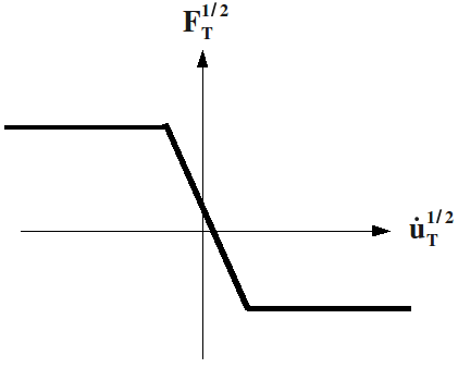
Graph of the law of friction approximated by penalization

Defining contact parameters

Here are the keywords used to define the parameters of contact, damping and friction in DEFI_MATERIAU [U4.43.01]:

• The RIGI_NOR operand allows you to give the value of the normal shock stiffness \({K}_{N}\).

• The AMOR_NOR operand allows you to give the value of the normal shock absorption \({C}_{N}\).

• The RIGI_TAN operand allows you to give the value of the tangential stiffness \({K}_{T}\).

• The AMOR_TAN operand allows you to give the value of the tangential shock damping \({C}_{T}\).

• The COULOMB operand is used to give the value of the Coulomb coefficient.

• The DIST_1 operand defines the characteristic distance of matter surrounding the first shock node.

• The DIST_2 operand defines the characteristic distance of material surrounding the second shock node (shock between two mobile structures).

• The operand JEU defines the distance between the shock node and an unmodelled obstacle (case of a shock between a mobile structure and an undeformable and immobile obstacle).

Internal variables

There are eight of them:

• \(V1\): displacement due to sliding in the tangential plane along the local \(y\) axis.

• \(V2\): displacement due to sliding in the tangential plane along the local \(z\) axis.

• \(V3\): speed along the local \(y\) axis.

• \(V4\): speed along the local \(z\) axis.

• \(V5\): component of the tangent force along the local axis \(y\): \({F}_{{cy}}\).

• \(V6\): component of the tangent force along the local axis \(z\): \({F}_{{cz}}\).

• \(V7\): management of the Coulomb criterion, adherent or sliding phase.

• \(V8\): displacement due to sliding in the tangential plane along the local \(x\) axis.