Nonlinear viscoelastic behavior DIS_VISC

Definition

Behavior DIS_VISC is a non-linear viscoelastic rheological behavior, of the extended Zener type, making it possible to schematize the behavior of a uniaxial shock absorber, only according to the local \(DX\) degree of freedom of discrete elements at two nodes (mesh SEG2) or and of discrete elements at one node (mesh) or and of discrete elements at one node (mesh POI1), in the case of a connection with a fixed non-meshed frame (see static and dynamic examples in the case of test SSND101). The arrangement of the linear elastic components makes it possible to take into account a wide range of environmental situations of the damping part of the device and its attachments.

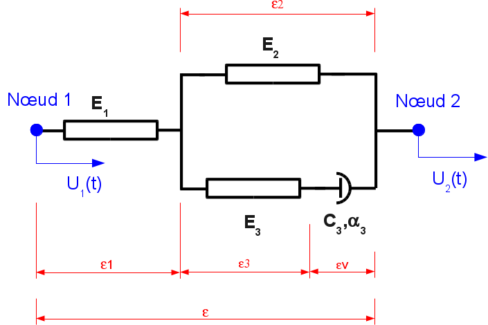
Discreet nonlinear viscoelastic rheological model.

The nonlinear viscous law is written, for \(\alpha \in \left]\mathrm{0,}1\right]\):

\({\sigma}_{3}\mathrm{=}E_3{\varepsilon}_{3}\mathrm{=}\mathit{C.}\mathit{sgn}({\dot{\varepsilon}}_{v}) . {∣{\dot{\varepsilon}}_{v}∣}^{\alpha }\)

[equ 6.1-1]

The damping constant \(C\) being positive. For \(\alpha =1\), the model is linear viscous. We note that the « time » dimension of this problem is, by the rules of similarity, directly associated with the coefficient \(C\): in fact, by noting the time reduced by \(\tau =\lambda t\), the nonlinear law is written: \({\sigma}_{3} = C . {\lambda}^{\alpha}\mathrm{sgn}({\dot{\varepsilon}}_{v}) . {∣\frac{{d\varepsilon}_{v}}{d\tau}∣}^{\alpha }\). Thus, considering a dynamic loading with a different pulsation (in relation \(\lambda\)) is the same as changing the coefficient \(C\) of the law in proportion to \({\lambda}^{\alpha }\). We note that case \(E_2\to \infty\) is not admissible, but we can choose \(E_2=0\) (pure serial system, type MAXWELL); similarly we will not take step \({E}_{1}\to \infty\) and \(E_3 \to \infty\) at the same time (model from KELVIN - VOIGT), otherwise the initial stiffness of the system would be infinite.

Formulation of behavior

Below, \(\varepsilon\) denotes the « deformation » of the discrete element, namely the difference in the axial displacements (direction \(x\) in the local coordinate system) of the nodes at the ends of the defined element:

\(\varepsilon ={U}_{x}^{\mathrm{N2}}-{U}_{x}^{\mathrm{N1}}\) on mesh SEG2 or \(\varepsilon ={U}_{x}^{\mathrm{N1}}\) on mesh POI1

[equ 6.2-1]

Likewise, the term \(\sigma\) denotes the « stress » of the discrete element below, namely the axial force transiting in the element defined on the SEG2 or POI1 mesh:

\(\sigma ={F}_{x}^{\mathrm{N2}}={F}_{x}^{\mathrm{N1}}\)

[equ 6.2-2]

The compatibility of the deformations gives, cf.:

\(\begin{cases}\varepsilon & = & \varepsilon_1+\varepsilon_2 \\ \varepsilon_2 & = & \varepsilon_3+\varepsilon_v\end{cases}\)

[equ 6.2-3]

The balance and the behavioral relationships give respectively (placing themselves below in the case \(\mathrm{sgn}({\dot{\varepsilon}}_{v})=+1\), for positive \(\varepsilon\) and \(\sigma\)):

\(\begin{cases}\sigma & = & E_1 \varepsilon_1 & ~ & \\ \sigma & = & \sigma_2 + \sigma_3 & = & E_2 \varepsilon_2+E_3 \varepsilon_3 \\ \sigma_3 & = & E_3 \varepsilon_3 & = & C.{\dot {\varepsilon}_v}^\alpha\end{cases}\)

[equ 6.2-4]

It is deduced respectively that:

\({\dot{\varepsilon}}_{2}={(\frac{{\sigma}_{3}}{C})}^{1/\alpha }+\frac{{\dot{\sigma}}_{3}}{E_3}\)	[equ 6.2-5]
\(\dot{\sigma}=E_2 . {(\frac{{\sigma}_{3}}{C})}^{1/\alpha }+\frac{{\dot{\sigma}}_{3}(E_2+E_3)}{E_3}\)	[equ 6.2-6]

And the evolution of the deformation is:

\(\dot{\varepsilon}=\frac{{E}_{1}+E_2}{{E}_{1}}{(\frac{{\sigma}_{3}}{C})}^{1/\alpha }+\frac{{\dot{\sigma}}_{2}({E}_{1}+E_2+E_3)}{{E}_{1}E_3}\)

[equ 6.2-7]

So the global law of behavior of the rheological system can be written in speed:

\(\dot{\sigma}=\frac{{E}_{1.}(E_2+E_3)\dot{\varepsilon}-{E}_{1}E_3 . {\dot{\varepsilon}}_{v}}{{E}_{1}+E_2+E_3}\)

[equ 6.2-8]

Speed \(\dot{\varepsilon}\) is calculated based on the movements and the time increment chosen:

\(\dot{\varepsilon}=({U}_{x}^{\mathrm{N2}}-{U}_{x}^{\mathrm{N1}})\text{/}\Delta t\)

It remains to express \({\dot{\varepsilon}}_{v}\) from the state variables:

\({\dot \varepsilon}_v={\left( \frac{1}{C} \left( \frac{\sigma \left(E_1+E_2 \right) } {E_1} - E_2 \varepsilon \right) \right) }^{1/\alpha}\)

[equ 6.2-9]

The elastic tangent speed stiffness of the model, which is used in the prediction phase, is:

\(K_t = \frac{E_1.(E_2+E_3)}{E_1+E_2+E_3} = \frac{1+E_2/E_3}{1/E_1+E_2/(E_1 . E_3)+1/E_3}\)

[equ 6.2-10]

The power dissipated is expressed by:

\({P}_{\mathrm{diss}}=C{\mid {\dot{\varepsilon}}_{v}\mid }^{1+\alpha }\)

[equ 6.2-11]

In the deformation-stress speed plane in the rheological model, for different values of \(\alpha\), the following cycles are observed:

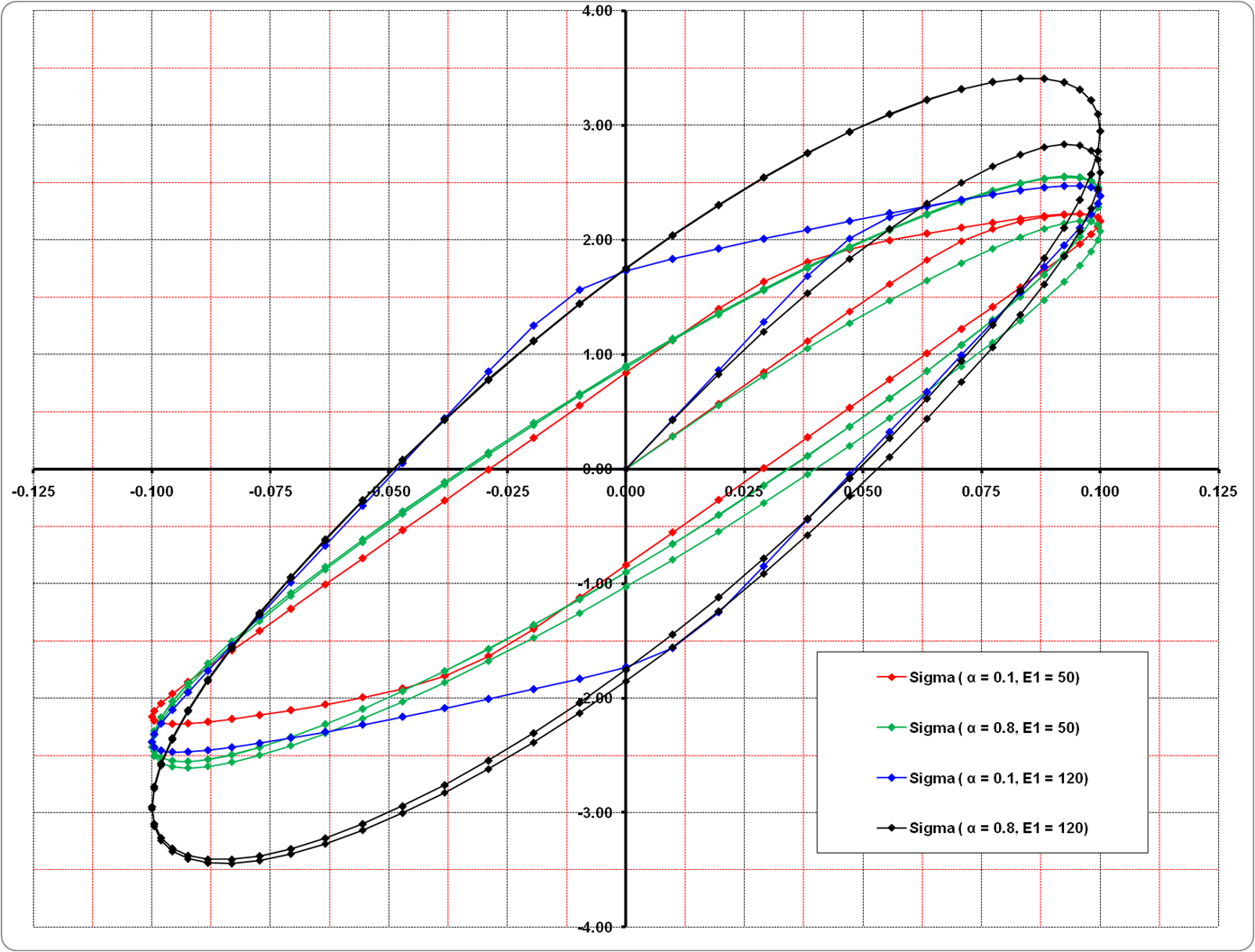
Response cycles of the discrete nonlinear viscoelastic rheological model (generalized Zener model). Force in Newton as a function of displacement in meters.

Note:

The inclination of the cycles comes from the effect of stiffness in parallel in the rheological behavior (Kelvin-Voigt or Zener) or in series (Maxwell model). In fact, in the case of a shock absorber alone without stiffness, the cycles are necessarily symmetric with respect to the zero displacement axis. If experimental curves of the behavior of such a damper device of this type are available, it will thus be possible, by recalibration, to determine the various coefficients of this law*DIS_VISC* . *

Data setting

The material coefficients are provided by the DIS_VISC keyword of the DEFI_MATERIAU command.

For the local direction \(x\) (and only that one) of the discrete element, 5 coefficients are provided, either the stiffness or the flexibility, then the damping characteristics:

• K1: elastic stiffness \(E_1\) of element 1 of the rheological model,

• K2: elastic stiffness \(E_2\) of element 2 of the rheological model,

• K3: elastic stiffness \(E_3\) of element 3 of the rheological model,

• UNSUR_K1: elastic flexibility \(1/E_1\) of element 1 of the rheological model,

• UNSUR_K2: elastic flexibility \(1/E_2\) of element 2 of the rheological model,

• UNSUR_K3: elastic flexibility \(1/E_3\) of element 3 of the rheological model,

• PUIS_ALPHA: power \(\alpha\) of the nonlinear law of the viscous behavior of the element,

• C: coefficient of the viscous behavior of the element.

The conditions to be met for these coefficients are (in particular to ensure the positivity and the finiteness of the tangent matrix):

\(E_1\ge {10}^{-8}\); \(1/E_1\ge 0\); \(E_3\ge {10}^{-8}\); \(1/E_3\ge 0\)

\(1/E_2\ge {10}^{-8}\); \(E_2\ge 0\); \(C\ge {10}^{-8}\); \({10}^{-8}\le \alpha \le 1\)

Moreover, we cannot have at the same time: \(1/E_1=0\), \(1/E_3=0\) and \(E_2=0\), that is to say the case of the shock absorber alone.

Integrating behavior

Local integration

An implicit EULER scheme is much less accurate (you would have to calculate the error in order 2) than a RUNGE - KUTTA diagram of order 5 with error control. Figure RK5 is a combination of the 4th order diagram and the 6th order diagram [bib9], for which the coefficients are determined so as to minimize the error between order 4 and order 6.

That’s why in*Code_Aster*, the local integration of this model uses the 5th order RUNGE - KUTTA schema. In addition, the tangent stiffness after discrete discretization in time of behavior \(\mathrm{dF}/\mathrm{dU}\) is obtained directly via the expression in the diagram RUNGE - KUTTA, at the end of the time step.

The error is known, so it is possible to trigger local subdivisions of the time step if the convergence criterion is not met.

Temporal integration and global balance

Moreover, if we consider the dynamic equilibrium of a system with one degree of freedom, of mass \(M\), including a shock absorber alone (without stiffness) obeying the law [eq], the equation of motion is written, having adopted the « reduced time » \(\tau =\lambda t\):

\(M\frac{{\mathrm{\partial }}^{2}u}{\mathrm{\partial }{\tau }^{2}}+\mathit{C.}{\lambda}^{2 - \alpha } . \mathit{sgn}(\frac{\mathrm{\partial }u}{\mathrm{\partial }\tau }) . {∣\frac{\mathrm{\partial }u}{\mathrm{\partial }\tau }∣}^{\alpha }\mathrm{=}0\)

[equ 6.4-1]

For example, let’s adopt the Newmark temporal integration scheme, cf. [R5.05.05], section§3.1; we note at the moment \({\tau }_{i}\) the quantities displacement, speed and acceleration: \({u}_{i}\), \({v}_{i}\), \({a}_{i}\) and \(\Delta \tau\) the « reduced time » step. So we have at moment \({\tau }_{i+1}\):

\(\begin{cases}{v}_{i+1} &=& \frac{\gamma}{\beta \Delta \tau }({u}_{i+1} - {u}_{i})+\frac{\beta - \gamma }{\beta}{v}_{i}+\frac{2\beta -\gamma }{2\beta}\Delta \tau . {a}_{i} \\{a}_{i+1} &=& \frac{1}{\beta \Delta {\tau }^{2}}({u}_{i+1} - {u}_{i})-\frac{1}{\beta \Delta \tau }{v}_{i}+\frac{2\beta - 1}{2\beta }.{a}_{i}\end{cases}\)

[equ 6.4-2]

Let’s inject these expressions [eq] to write the balance [eq] at time \({\tau }_{i+1}\), in case \({v}_{i}\ge 0\), expanded to the first order in \(\Delta v\):

\(\stackrel{ˆ}{K}{u}_{i+1}=\frac{M{u}_{i}}{\beta \Delta {\tau }^{2}}+\frac{M{v}_{i}}{\beta \Delta \tau }-\frac{2\beta -1}{2\beta } . M{a}_{i}+\mathrm{C.}{\lambda}^{2-\alpha } . {(\frac{\beta -\gamma }{\beta }{v}_{i}+\frac{2\beta -\gamma }{2\beta }\Delta \tau . {a}_{i})}^{1-\alpha }\)

[equ 6.4-3]

the tangent matrix being:

\(\stackrel{ˆ}{K}=\frac{M}{\beta \Delta {\tau }^{2}}+\frac{\alpha \gamma \mathrm{C.}{\lambda}^{2-\alpha }}{\beta \Delta \tau } . {(\frac{\beta -\gamma }{\beta }{v}_{i}+\frac{2\beta -\gamma }{2\beta }\Delta \tau . {a}_{i})}^{\alpha -1}\)

[equ 6.4-4]

In case \(\alpha =1\) (linear damper), we find the tangent matrix \(\stackrel{ˆ}{K}\) and the dependence on the time step \(\Delta t\) usual in the Newmark diagram for the linear case, cf. [R5.05.05].

In the case \(\alpha \ne 1\) (non-linear damper), it is observed that \({v}_{i}\) and \({a}_{i}\) cannot be zero together (except in static terms), the tangent matrix \(\stackrel{ˆ}{K}\) of the Newmark diagram sees its dependence on the time step affected by the factor \(\mathrm{C.}{\lambda}^{2-\alpha }\). So if we vary the coefficient \(C\) of the law, we will have to vary the time step of temporal integration. It is also possible to adopt a technique for subdividing the time step, cf. operator STAT_NON_LINE [U4.51.03] and operator DYNA_NON_LINE [U4.53.01].

This discrete element behavior model is also available identically within operators DYNA_VIBRA [U4.53.03] and DYNA_TRAN_MODAL [U4.53.21], for dynamic analysis on a modal basis with nonlinearities located on nodes, and time integration schemes for Euler or Runge-Kutta dynamics of order 5 and 3 order, at adaptive steps. It is integrated locally at the same time in the same way, see Intégration locale. As in dynamics on a physical basis, we must define the time step of the diagram according to the parameters of law DIS_VISC, whose values are defined directly in the operators DYNA_VIBRA and DYNA_TRAN_MODAL.

Internal variables

Behavior DIS_VISC has 4 internal variables:

• \(V1\): FORCE: contains the effort \(\sigma\) at every moment in the rheological model.

• \(V2\): UVISQ: viscous displacement of the shock absorber \({\varepsilon}_{v}\).

• \(V3\): DISSTHER: contains the dissipated energy updated at each moment:

  \(\mathrm{V3}=\sum \mid \frac{{\sigma}^{\text{+}}(E_1+E_2)}{E_1}-E_2{\varepsilon}^{\text{+}}\mid . \mid {\varepsilon}_{v}^{\text{+}}-{\varepsilon}_{v}^{\text{-}}\mid\)

• \(V4\): RAIDEUR: stiffness tangent to behavior \(\mathrm{dF}/\mathrm{dU}\).