Behavior JONC_ENDO_PLAS#
Definition#
Behavior JONC_ENDO_PLAS is used to model on discrete elements (ball joints), of type DIS_TR on cells SEG2, at two nodes, the nonlinear behavior of a connection in out-of-plane bending, cf. [U2.02.03]. This model was designed to treat the junction between a wall and a floor or a slab, made of reinforced concrete, modelled in plate finite elements, or even in solid finite elements. The nonlinear relationship is expressed in the moment \(M\) - relative rotation \(\theta\) plane along the local axis \(\mathit{Oz}\). This behavior model was developed as part of [bib10], [bib11].
The implementation is described on the: sectional view and perspective view. \(\mathit{SH}\) refers to the core of the junction, which is modelled by a linear finite element, on a hexahedral mesh with eight knots, on which linear elastic behavior has been assigned — see [U2.03.10] — and \(\mathit{FL}\) refers to the discrete elements with two nodes, supports the law of behavior JONC_ENDO_PLAS. The latter should be understood as the « condensation » along the junction edge of the linear contributions of moments transmitted by the two linked structural elements (wall, floor).
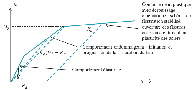
The phenomenology, cf., of the junction behavior model is initially elastic, then damaging (stiffness degradation), and finally integrates plastic behavior (irreversible rotational deformations) to describe the observed phenomena, cf.. A distinction is made between « positive » and « negative » rotation paths, for which degradation may occur non-symmetrically depending on the characteristics of the sections.
sectional view, plan \((x,y)\) |
perspective view |
|
Implementation of the discrete nonlinear model in flexure of a junction between two walls and two floors (current situation) . |
||
Phenomenology results from situations schematised on the following.
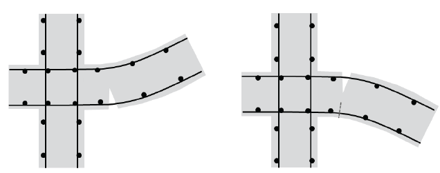
Diagram showing the opening of a crack in positive bending in the floor (on the left) then its closure and the opening of a second crack in negative bending (on the right).#
Discreet nonlinear rheological model in vail-floor junction flexure.#
Parameters of the law of behavior#
There are eight of them (real positives all mandatory, cf. [U4.43.01]):
KE: stiffness in elastic rotation \({K}_{e}>0\);
KP: plastic work hardening slope \({K}_{p}\le {K}_{e}\);
KDP: tangent stiffness \({K}_{d}^{\text{+}}\in \left[{K}_{e},{K}_{p}\right]\) in the damaging phase for positive bending,
KDM: tangent stiffness \({K}_{d}^{\text{-}}\in \left[{K}_{e},{K}_{p}\right]\) in the damaging phase for negative bending,
RDP: rotation damage threshold \({\theta }_{d}^{\text{+}}>0\) in positive bending,
RDM: rotation damage threshold \({\theta }_{d}^{\text{-}}<0\) in negative bending,
MYP: plasticity threshold \({M}_{y}^{\text{+}}\) in positive flexure,
MYM: plasticity threshold \({M}_{y}^{\text{-}}\le {K}_{e}{\theta }_{d}^{\text{-}}\) in negative flexure.
In [bib10] §3.5., and [bib11], we describe how to determine the parameters from the analysis of the reinforced concrete section: geometry and characteristics of the materials. The hypothesis of an elastic linear behavior of concrete up to the crack threshold is preferred. In compression, the hypothesis of perfect elastoplastic behavior of concrete is retained in accordance with EN1992 -1-1. Steels are supposed to be elastoplastic.
As this is a behavior model for a discrete element, a reference length is assigned along the \(\mathrm{Oz}\) axis of the junction: the moments \(M\) are therefore understood in units of torque (distance * force).
Formulation of the law of behavior#
In the following, we denote the parts positive (or negative) of a scalar quantity by:
\({\langle x\rangle }_{\text{+}}=\mathrm{Max}(\mathrm{0,}x)\); \({\langle x\rangle }_{\text{-}}=\mathrm{Max}(\mathrm{0,}-x)\) |
[equ 15.3-1] |
This behavior model is formulated within the framework of the thermodynamics of irreversible processes. The primary state variables for this behavior model are:
\(\theta\) the total differential rotation (along the local \(\mathrm{Oz}\) axis) on either side of the junction,
\({\theta }^{p}\) the relative plastic rotation of the junction,
\({D}^{\text{+}}\) scalar damage, which represents degradation following the initiation of a crack from the underside, evolving according to the sign of the moment on the reinforced concrete section,
\({D}^{\text{-}}\) scalar damage, which represents degradation following the initiation of a crack from the upper face, evolving according to the sign of the moment on the reinforced concrete section,
\(\alpha\) the kinematic work hardening variable.
Free energy is written as:
\(\phi (\theta ,{\theta }^{p},{D}^{\text{+}},{D}^{\text{-}},\alpha )=\frac{1}{2}{\tilde{K}}_{e}^{\text{+}}({D}^{\text{+}}){\langle \theta -{\theta }^{p}\rangle }_{\text{+}}^{2}+\frac{1}{2}{\tilde{K}}_{e}^{\text{-}}({D}^{\text{-}}){\langle \theta -{\theta }^{p}\rangle }_{\text{-}}^{2}+\frac{1}{2}{K}_{p}{\alpha }^{2}\) |
[equ 15.3-2] |
with respectively:
\({\tilde{K}}_{e}^{\text{+/-}}({D}^{\text{+/-}})={K}_{e}(1-{D}^{\text{+/-}})\) with \({D}^{\text{+}}\in \left[\mathrm{0,}1\right[\) and \({D}^{\text{-}}\in \left[\mathrm{0,}1\right[\) |
[equ 15.3-3] |
where the elastic stiffness parameter \({K}_{e}\) has been defined, cf.
The first state law of the model is derived from]:
\(M={\phi }_{,\theta }={\tilde{K}}_{e}^{\text{+}}({D}^{\text{+}}){\langle \theta -{\theta }^{p}\rangle }_{\text{+}}-{\tilde{K}}_{e}^{\text{-}}({D}^{\text{-}}){\langle \theta -{\theta }^{p}\rangle }_{\text{-}}\) |
[equ 15.3-4] |
The thermodynamic forces associated with the internal variables of the model are respectively:
\(\{\begin{array}{}{M}_{p}=-{\phi }_{,{\theta }^{p}}={\tilde{K}}_{e}({D}^{\text{+}}){\langle \theta -{\theta }^{p}\rangle }_{\text{+}}-{\tilde{K}}_{e}({D}^{\text{-}}){\langle \theta -{\theta }^{p}\rangle }_{\text{-}}=M\\ {Y}^{\text{+}}=-{\phi }_{,{D}^{\text{+}}}=\frac{1}{2}{K}_{e}\mathrm{.}{\langle \theta -{\theta }^{p}\rangle }_{\text{+}}^{2}\\ {Y}^{\text{-}}=-{\phi }_{,{D}^{\text{-}}}=\frac{1}{2}{K}_{e}\mathrm{.}{\langle \theta -{\theta }^{p}\rangle }_{\text{-}}^{2}\\ X=-{\phi }_{,\alpha }=-{K}_{p}\alpha \end{array}\) |
[equ 15.3-5] |
where we defined the plastic work hardening slope parameter \({K}_{p}\), cf.
The instantaneous intrinsic dissipation in any admissible evolution is then written as:
\({D}_{\mathrm{diss}}={M}_{p}\mathrm{.}\dot{{\theta }^{p}}+{Y}^{\text{+}}\mathrm{.}\dot{{D}^{\text{+}}}+{Y}^{\text{-}}\mathrm{.}\dot{{D}^{\text{-}}}+X\mathrm{.}\dot{\alpha }\) |
[equ 15.3-6] |
either:
\(\begin{array}{}{D}_{\mathrm{diss}}={\tilde{K}}_{e}^{\text{+}}({D}^{\text{+}}){\langle \theta -{\theta }^{p}\rangle }_{\text{+}}\mathrm{.}{\dot{\theta }}^{p}-{\tilde{K}}_{e}^{\text{-}}({D}^{\text{-}}){\langle \theta -{\theta }^{p}\rangle }_{\text{-}}\mathrm{.}{\dot{\theta }}^{p}\\ +\frac{1}{2}{K}_{e}\mathrm{.}{\langle \theta -{\theta }^{p}\rangle }_{\text{+}}^{2}\mathrm{.}\dot{{D}^{\text{+}}}+\frac{1}{2}{K}_{e}\mathrm{.}{\langle \theta -{\theta }^{p}\rangle }_{\text{-}}^{2}\mathrm{.}\dot{{D}^{\text{-}}}-{K}_{p}\mathrm{.}\alpha \mathrm{.}\dot{\alpha }\end{array}\) |
[equ 15.3-7] |
In any acceptable evolution, \(\dot{{D}^{\text{-}}}\) and \(\dot{{D}^{\text{+}}}\) are positive or zero: the damage can only increase.
Two intermediate rotation variables are used in positive and negative bending:
\({\theta }^{\text{+}}=\mathrm{Max}({\langle \theta -{\theta }^{p}\rangle }_{\text{+}},{\theta }_{d}^{\text{+}})\) \({\theta }^{\text{-}}=\mathrm{Max}({\langle \theta -{\theta }^{p}\rangle }_{\text{-}},\mid {\theta }_{d}^{\text{-}}\mid )\) |
[equ 15.3-8] |
to simplify the writing of the increments of the plastic damage and rotation variables.
In a monotonic loading path increasing in positive or negative bending, we directly obtain:
\(\{\begin{array}{}\dot{{D}^{\text{+}}}=0\mathrm{pour}\mid \theta -{\theta }^{p}\mid \le {\theta }_{d}^{\text{+}}\\ \dot{{D}^{\text{-}}}=0\mathrm{pour}\mid \theta -{\theta }^{p}\mid \le {\theta }_{d}^{\text{-}}\\ {D}^{\text{+}}=(1-\frac{{K}_{d}^{\text{+}}}{{K}_{e}})\mathrm{.}(1-\frac{{\theta }_{d}^{\text{+}}}{{\theta }^{\text{+}}})\mathrm{pour}\mid \theta -{\theta }^{p}\mid >{\theta }_{d}^{\text{+}}\\ {D}^{\text{-}}=(1-\frac{{K}_{d}^{\text{-}}}{{K}_{e}})\mathrm{.}(1-\frac{\mid {\theta }_{d}^{\text{-}}\mid }{{\theta }^{\text{-}}})\mathrm{pour}\mid \theta -{\theta }^{p}\mid >{\theta }_{d}^{\text{-}}\end{array}\) |
[equ 15.3-9] |
where we defined four parameters to be identified on a positive charge path, cf., then a negative charge path:
\({K}_{d}^{\text{+}}\in \left[{K}_{e},{K}_{p}\right]\), \({K}_{d}^{\text{-}}\in \left[{K}_{e},{K}_{p}\right]\), \({\theta }_{d}^{\text{+}}>0\) and \({\theta }_{d}^{\text{-}}>0\) |
[equ 15.3-10] |
The last two parameters, without units, correspond to the relative rotation observed at the beginning of the flexural cracking of the reinforced concrete section at the junction, under positive charge, then under negative charge.
The following two damage threshold functions are therefore compatible with this type of directly integrated evolution:
\({f}_{({Y}^{\text{+}};{D}^{\text{+}})}^{d\text{+}}={\tilde{f}}_{({\theta }^{p},{D}^{\text{+}})}^{d\text{+}}=\sqrt{\frac{2\mathrm{.}{Y}^{\text{+}}}{{K}_{e}}}\mathrm{.}(1-\frac{{K}_{e}\mathrm{.}{D}^{\text{+}}}{{K}_{e}-{K}_{d}^{\text{+}}})-{\theta }_{d}^{\text{+}}={\langle \theta -{\theta }^{p}\rangle }_{\text{+}}\mathrm{.}(1-\frac{{K}_{e}\mathrm{.}{D}^{\text{+}}}{{K}_{e}-{K}_{d}^{\text{+}}})-{\theta }_{d}^{\text{+}}\le 0\) |
[equ 15.3-11] |
\({f}_{({Y}^{\text{-}};{D}^{\text{-}})}^{d\text{-}}={\tilde{f}}_{({\theta }^{p},{D}^{\text{-}})}^{d\text{-}}=\sqrt{\frac{2\mathrm{.}{Y}^{\text{-}}}{{K}_{e}}}\mathrm{.}(1-\frac{{K}_{e}\mathrm{.}{D}^{\text{-}}}{{K}_{e}-{K}_{d}^{\text{-}}})-\mid {\theta }_{d}^{\text{-}}\mid ={\langle \theta -{\theta }^{p}\rangle }_{\text{-}}\mathrm{.}(1-\frac{{K}_{e}\mathrm{.}{D}^{\text{-}}}{{K}_{e}-{K}_{d}^{\text{-}}})-\mid {\theta }_{d}^{\text{-}}\mid \le 0\) |
[equ 15.3-12] |
while respecting Kuhn-Tucker conditions and the positivity of the dissipation.
The two plastic flow threshold functions are respectively defined by:
\({f}^{p\text{+/-}}(M;X)={\langle M-X\rangle }_{\text{+/-}}-{M}_{y}^{\text{+/-}}\le 0\) |
[equ 15.3-13] |
with two plasticity threshold parameters \({M}_{y}^{\text{+}}\) and \({M}_{y}^{\text{-}}\) to be identified on a positive charge path then a negative charge path.
The law of plastic flow is written (rule of normality), with \({\dot{\lambda }}^{p}\ge 0\) and \({\dot{\lambda }}^{p}\mathrm{.}{f}^{p\text{+/-}}(M;X)=0\):
\({\dot{\theta }}^{p}=\dot{\alpha }={\dot{\lambda }}^{p}\mathrm{.}{f}_{,M}^{p}={\dot{\lambda }}^{p}\mathrm{.}\mathrm{sgn}(M-X)=-{\dot{\lambda }}^{p}\mathrm{.}{f}_{,X}^{p}\) |
[equ 15.3-14] |
which, in particular, ensures:
\(\dot{M}=\dot{X}={K}_{p}\mathrm{.}\dot{\alpha }={K}_{p}\mathrm{.}{\dot{\theta }}^{p}\) |
[equ 15.3-15] |
From the equations] and], a simpler expression for instantaneous intrinsic dissipation] is deduced:
\({D}_{\mathrm{diss}}=(M-X)\mathrm{.}{\dot{\theta }}^{p}+\frac{1}{2}{K}_{e}\mathrm{.}{\langle \theta -{\theta }^{p}\rangle }_{\text{+}}^{2}\mathrm{.}\dot{{D}^{\text{+}}}+\frac{1}{2}{K}_{e}\mathrm{.}{\langle \theta -{\theta }^{p}\rangle }_{\text{-}}^{2}\mathrm{.}\dot{{D}^{\text{-}}}\) |
[equ 15.3-16] |
the term \((M-X)\mathrm{.}{\dot{\theta }}^{p}=\mid {{M}_{y}^{\text{+/-}}\mathrm{.}\dot{\theta }}^{p}\mid\) being itself obtained by the value reached by the plastic threshold \({M}_{y}^{\text{+/-}}\) according to the sign of \((M-X)\), cf.], and the contributions of the damage using].
The moment-rotation responses of this model for a cyclic loading path of increasing amplitude, not alternating and then alternating, are presented in the.
not alternate |
alternate |
Response of the nonlinear veil-floor junction flexure model for a loading of increasing amplitude |
|
Local digital integration of the law of behavior#
The numerical scheme for the temporal integration of the law is based on the method of RUNGE - KUTTA of order 5 with error control and division. Figure RK5 is a combination of the 4th order diagram and the 6th order diagram [bib9], for which the coefficients are determined so as to minimize the error between order 4 and order 6. The convergence tolerance is defined by the value of RESI_INTE_RELA.
The seven nonlinear equations to be solved by diagram RK5 are:
the current state relationship \(M\), cf.];
the relationship giving the differential rotation \(\theta\);
the relationship giving plastic rotation \({\theta }^{p}\);
the relationship giving \({D}^{\text{+}}\), cf.];
the relationship giving \({D}^{\text{-}}\), cf.];
the relationship giving \(X\), cf.];
the relationship giving \({D}_{\mathrm{diss}}\), cf.].
The secant operator (scalar \(\Delta M/\Delta \theta\)) is then returned to the general nonlinear equilibrium integration scheme.
The error is known, so it is possible to trigger local subdivisions of the time step if the convergence criterion is not met.
The two intermediate rotation variables, cf.], are initialized by: \({\theta }^{\text{+}}({t}_{0})={\theta }_{d}^{\text{+}}\) and \({\theta }^{\text{-}}({t}_{0})=\mid {\theta }_{d}^{\text{-}}\mid\).
Numerical integration verification is available in test case SSND114 [V6.08.114].
Internal variables#
There are nine of them:
\(V\mathrm{1}\): differential rotation \({\theta }_{2}-{\theta }_{1}\) on the discrete element, along the local axis \(\mathrm{Oz}\), named ROTATOTA.
\(V\mathrm{2}\): plastic rotation \({\theta }^{p}\) (along the local axis \(\mathrm{Oz}\)), named ROTAPLAS,
\(V\mathrm{3}\): intermediate variable of rotation in positive bending \({\theta }^{\text{+}}\), cf.], named ROTAPLUS,
\(V\mathrm{4}\): intermediate variable of rotation in negative flexure \({\theta }^{\text{-}}\), cf.], named ROTAMOIN,
\(V\mathrm{5}\): return moment variable associated with kinematic work hardening \(X={K}_{p}\mathrm{.}\alpha\), named XCIN_MZZ,
\(V\mathrm{6}\): instantaneous dissipation \({D}_{\mathrm{diss}}\) (plastic damage and work hardening mechanisms), named DISSTOTA,
\(V\mathrm{7}\): internal damage variable \({D}^{\text{+}}\) in the lower wall (positive flexure), named ENDOPLUS,
\(V\mathrm{8}\): internal damage variable \({D}^{\text{-}}\) in the upper wall (negative flexure), named ENDOMOIN,
\(V\mathrm{9}\): variable for initializing damage thresholds (activated at the first time step), named INISEUIL.