Behavior DIS_ECRO_CINE

Definition

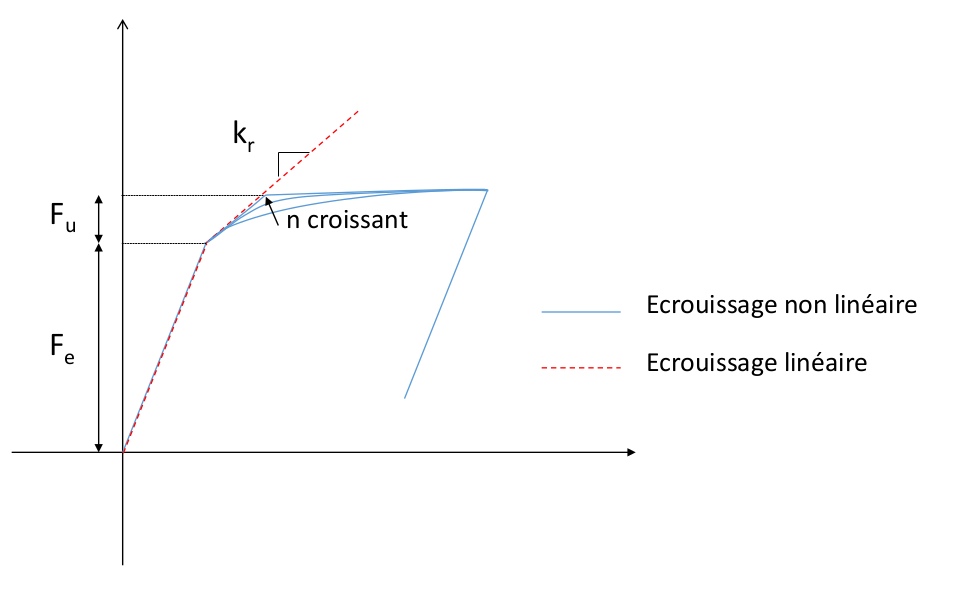
Behavior DIS_ECRO_CINE is a law of elastoplastic behavior with nonlinear kinematic work hardening for discrete elements. This law is defined for each component of the torsor of the resulting efforts. Material coefficients are provided under the keyword DIS_ECRO_CINE.

For example for direction \(X\):

• LIMY_DX: \({F}_{e}\) Elastic limit force along the local \(x\) axis of the element

• KCIN_DX: \({k}_{r}\) Stiffness along the local \(x\) axis of the element

• PUIS_DX: \(n\) Non-linearity coefficient along the local axis \(x\) of the element (greater than 1)

• LIMU_DX: \({F}_{u}\) Difference between the limit force and the elastic limit force along the local \(x\) axis of the element.

  • Threshold: :math: `f=left|f-Xright|- {F} _ {e} `

    • If \(f\le 0\) the behavior is elastic \(\dot{F}={K}_{e}.\dot{U}\)

    • If not:

\(\begin{array}{l}f=0~~et~~\dot{f}=0 \\ \dot{{U}^{\mathrm{an}}}=\dot{\lambda }\frac{\partial f}{\partial F}-\dot{\alpha }=\dot{\lambda }\frac{\partial f}{\partial X}\end{array}\)	[equ 3.1-1]
\(\dot{F}={K}_{e}(\dot{U}-\dot{{U}^{\mathrm{an}}})\)	[equ 3.1-2]

Law DIS_ECRO_CINE: Parameter Description

\(X=\frac{{k}_{\mathrm{r.}}\alpha }{{(1+{(\frac{{k}_{\mathrm{r.}}\alpha }{{F}_{u}})}^{n})}^{\frac{1}{n}}}\)

[equ 3.1-3]

It is pointed out that this law of behavior is not compatible with alternating cyclic loading.

Integrating behavior

The resolution is obtained after time discretization in the following way:

\(\Delta F={K}_{e}(\Delta U-\Delta {U}^{\mathrm{an}})\) where \(\Delta F,\Delta U\) can represent either efforts and translations, or moments and rotations.

By calculating: \({F}^{\text{-}}={K}_{e}({U}^{\text{-}}-{U}_{\mathrm{an}}^{\text{-}})\), an elastic test is carried out:

If \(∣{F}^{\text{-}}+{K}_{e}(\Delta U)-{X}^{\text{-}}∣\le 0\) then \(\Delta F={K}_{e}.\Delta U\)

If not, the system to be solved is:

\(\begin{array}{l}f=0\Rightarrow ∣{F}^{\text{-}}+\Delta F-{X}^{\text{-}}-\Delta X∣={F}_{e}\\ \Delta {U}^{\mathrm{an}}=\Delta \alpha =\Delta \lambda \frac{{F}^{\text{-}}+\Delta F-{X}^{\text{-}}-\Delta X}{{F}_{e}}\\ \Delta F={K}_{e}(\Delta U-\Delta {U}^{\mathrm{an}})\end{array}\)

[equ 3.2-1]

The 3 unknowns are: \(\Delta F;\Delta {U}^{\mathrm{an}}=\Delta \alpha ;\Delta \lambda\) because \(\Delta X=\frac{k({\alpha }^{\text{-}}+\Delta \alpha )}{{(1+{(k({\alpha }^{\text{-}}+\Delta \alpha ))}^{n})}^{1/n}}-{X}^{\text{-}}\) is an analytic function of \(\Delta \alpha\).

This system can be simplified in the following way:

\(\begin{array}{l}∣{F}^{\text{-}}+\Delta F\mathrm{-}{X}^{\text{-}}\mathrm{-}\Delta X∣\mathrm{=}{F}_{e}\\ \Delta {U}^{\mathit{an}}\mathrm{=}\Delta \lambda \frac{{F}^{\text{-}}+\Delta F\mathrm{-}{X}^{\text{-}}\mathrm{-}\Delta X}{{F}_{e}}\\ \Delta F+{F}^{\text{-}}\mathrm{-}{X}^{\text{-}}\mathrm{-}\Delta X\mathrm{=}{K}_{e}(\Delta U\mathrm{-}\Delta {U}^{\mathit{an}})+{F}^{\text{-}}\mathrm{-}{X}^{\text{-}}\mathrm{-}\Delta X\end{array}\)

So:

\(\begin{array}{l}∣{F}^{\text{-}}+\Delta F\mathrm{-}{X}^{\text{-}}\mathrm{-}\Delta X∣\mathrm{=}{F}_{e}\\ \Delta {U}^{\mathit{an}}\mathrm{=}\Delta \lambda \frac{{F}^{\text{-}}+\Delta F\mathrm{-}{X}^{\text{-}}\mathrm{-}\Delta X}{{F}_{e}}\\ \Delta F+{F}^{\text{-}}\mathrm{-}{X}^{\text{-}}\mathrm{-}\Delta X\mathrm{=}{K}_{e}\Delta U+{F}^{\text{-}}\mathrm{-}{X}^{\text{-}}\mathrm{-}\Delta X\mathrm{-}{K}_{e}\Delta \lambda \frac{{F}^{\text{-}}+\Delta F\mathrm{-}{X}^{\text{-}}\mathrm{-}\Delta X}{{F}_{e}}\end{array}\)

[equ 3.2-2]

The last equation provides:

\((\Delta F+{F}^{\text{-}}-{X}^{\text{-}}-\Delta X)(1+{K}_{e}\Delta \frac{\lambda }{{F}_{e}})={K}_{e}\Delta U+{F}^{\text{-}}-{X}^{\text{-}}-\Delta X\) where \(\Delta X\) is a function of \(\Delta \alpha\) and therefore of \(\Delta \lambda\) (and the sign of \(F-X\)). Taking the norm to the right and to the left we get:

\({F}_{e}+{K}_{e}\Delta \lambda =\mid {K}_{e}\Delta U+{F}^{\text{-}}-{X}^{\text{-}}-\Delta X\mid\)

This unique scalar equation can be solved by a classical method of finding zero functions (Newton, secant, etc. see for example [R5.03.04]). In the case where kinematic work hardening is linear, (the only case justified thermodynamically [bib8]), the solution \(\Delta \lambda\): \({F}_{e}+({K}_{e}+k)\Delta \lambda =\mid {K}_{e}\Delta U+{F}^{\text{-}}-{X}^{\text{-}}\mid\) is obtained analytically.

The other unknowns are then calculated by:

\(\Delta F=\frac{{K}_{e}\Delta U+{F}^{\text{-}}-{X}^{\text{-}}-\Delta X}{(1+{K}_{e}\frac{\Delta \lambda }{{F}_{e}})}-{F}^{\text{-}}+{X}^{\text{-}}+\Delta X\) and \(\Delta {U}^{\mathrm{an}}=\Delta \lambda \frac{{F}^{\text{-}}+\Delta F-{X}^{\text{-}}-\Delta X}{{F}_{e}}\)

The current programming solves the system in a simplified way:

\(f=∣F-X∣-{F}_{e}\) is discretized explicitly: \(f=∣F-{X}^{\text{-}}∣-{F}_{e}\)

so: \({F}_{e}+{K}_{e}\Delta \lambda =\mid {K}_{e}\Delta U+{F}^{\text{-}}-{X}^{\text{-}}\mid\).

We then calculate \(\alpha \mathrm{=}{\alpha }^{\text{-}}+\Delta {U}^{\mathit{an}}\), which allows us to update: \(X=\frac{{k}_{\mathrm{r.}}\alpha }{{(1+{(\frac{{k}_{\mathrm{r.}}\alpha }{{F}_{u}})}^{n})}^{\frac{1}{n}}}\).

The tangent stiffness in this direction is approximated by:

\({K}_{\mathrm{tgt}}=\frac{\Delta F}{\Delta U}\)

[equ 3.2-3]

Internal variables

There are 3 internal variables per degree of freedom:

• \(V1\) contains \({U}^{\mathrm{an}}\) at all times

• \(V2\) contains \(\alpha\) at all times

• \(V3\) contains the total energy updated at any moment.