4. Implementation in Code_Aster#

4.1. Resolution algorithm#

The algorithm used is of the global-local type.

Global iterations use the elastic stiffness matrix calculated from the damaged Hooke matrix:

\(\underline{\underline{\underline{\underline{\Lambda }}}}=(1-D){\underline{\underline{\underline{\underline{\Lambda }}}}}^{0}\)

At the level of local iterations (i.e. at each point in GAUSS), the numerical integration of the speed equations can be carried out either by an explicit Runge-Kutta scheme of order 2 with automatic division into local sub-steps according to an estimate of the integration error (nested Runge-Kutta method), or by an implicit Euler diagram solved by a Newton method. Refer to references [bib3] for all the details concerning numerical methods, and to [R5.03.14] for the explicit algorithms used and their computer programming.

4.2. Implicit integration of the behavioral relationship#

At each global iteration of solving the variational balance problem and for each elementary integration point, it is necessary to integrate the equations of the model described in [§3] to obtain the stress tensor and possibly calculate the tangent behavior operator.

The problem written in generic form at time t consists of the following four systems of nonlinear equations:

\(\mathrm{\{}\begin{array}{c}\underline{\text{Rb}}(\underline{\beta },\underline{p},\underline{\varepsilon },{\underline{\nu }}_{\text{etat}}^{t\mathrm{-}1})\mathrm{=}\underline{0}\\ \underline{\text{Rp}}(\underline{\beta },\underline{p},\underline{\varepsilon },{\underline{\nu }}_{\text{etat}}^{t\mathrm{-}1})\mathrm{=}\underline{0}\end{array}\) eq 4.2-1

with

\(\{\begin{array}{}\underline{\Omega }(\underline{\underline{\sigma }},\underline{\beta },\underline{p},\underline{\varepsilon },{\underline{\nu }}_{\text{etat}}^{t-1})=\underline{0}\\ \underline{\Theta }({\underline{\nu }}_{\text{etat}},\underline{\beta },\underline{p},\underline{\varepsilon },{\underline{\nu }}_{\text{etat}}^{t-1})=\underline{0}\end{array}\) eq 4.2-2

\(\underline{\text{Rb}}\) is a system of six equations (six unknowns) describing the unknowns associated with constraints. The 6-component vector of these unknowns is denoted \(\underline{\beta }\). The link between \(\underline{\beta }\) and \(\underline{\underline{\sigma }}\) is achieved using the system of equations \(\underline{\Omega }\) and the vector \(\underline{p}\) contains the variables \(r\) and \(D\).

\(\underline{\text{Rp}}\) is a system of equations describing internal unknowns. We opt for a system of 2 equations with \(\dot{D}\) and \(\dot{r}\) as internal unknowns. The evolution of state variables is described by the system of equations \(\underline{\Theta }\).

The implicit Euler schema is used and the algorithm takes the following form:

Initialization of the unknowns of the discretized problem and recovery of the values of the state variables obtained at the previous step

iterations of the Newton method (maximum number of iterations pre-defined by the user): 1. Retrieving the values of the parameters involved in the material law (the elasticity operator) 2. Calculation of stress criteria and their derivatives with respect to stresses 3. Retrieving the values of the parameter k involved in the evolution of the damage and its derivative 4. Calculation of the current value of state variables, equations describing internal unknowns, and equations describing constraints 5. Calculation of the derivatives of equations with respect to the unknowns 6. Linear system resolution \(\left[\begin{array}{cc}{\frac{\partial \underline{\text{Rb}}}{\partial \underline{\beta }}}^{n}& {\frac{\partial \underline{\text{Rb}}}{\partial \underline{p}}}^{n}\\ {\frac{\partial \underline{\text{Rp}}}{\partial \underline{\beta }}}^{n}& {\frac{\partial \underline{\text{Rp}}}{\partial \underline{p}}}^{n}\end{array}\right]\left[\begin{array}{c}\underline{d\beta }\\ \underline{\mathrm{dp}}\end{array}\right]=-\left[\begin{array}{c}{\underline{\text{Rb}}}^{n}\\ {\underline{\text{Rp}}}^{n}\end{array}\right]\) eq 4.2-3 * Convergence test

Evaluation of the tangent operator

4.2.1. Implicit discretization of model equations#

Considering that an increment of time characterizes a new state of the system [éq 4.2-1] and [éq 4.2-2] solved by a Newton algorithm, we choose to identify the state of a quantity at the previous moment by the exponent t-1 while its current state is noted without an exponent. Thus, the variation of a quantity for the time increment in question is presented by \(U={U}^{t-1}+\Delta U={U}^{t-1}+\Delta t\dot{U}(\theta \Delta t)\).

For \(\theta =0\), you get an explicit schema and for \(\theta =1\), you get a purely implicit schema.

With these notations, the discretized form of the vector system is written:

\(\underline{\text{Rb}}\equiv \underline{\beta }-(1-({D}^{t-1}+\Delta t\dot{D}))\underline{\underline{\Lambda }}(\underline{\varepsilon }-{\underline{\varepsilon }}_{\text{th}}-({\underline{\varepsilon }}_{\text{vp}}^{t-1}+\Delta t\frac{3}{2}\dot{r}\frac{\underline{{\sigma }^{\text{'}}}(\underline{\beta })}{(1-({D}^{t-1}+\Delta t\dot{D})){\sigma }_{\text{eq}}(\underline{\beta })}))=\underline{0}\) eq 4.2.1-1

or more simply \(\underline{\text{Rb}}\equiv \underline{\beta }-(1-({D}^{t-1}+\Delta t\dot{D}))\underline{\underline{\Lambda }}{\underline{\varepsilon }}_{\text{el}}=\underline{0}\)

\(\underline{\Omega }\equiv \underline{\sigma }=\underline{\beta }\)

where \(\underline{\beta }\) is the 6-component vector from the \(\underline{\underline{\sigma }}\) stress tensor.

\(\underline{\text{Rp}}\equiv \{\begin{array}{}\dot{r}-{\langle \frac{{\sigma }_{\text{eq}}(\underline{\beta })-{\sigma }_{y}(1-({D}^{t-1}+\Delta t\dot{D}))}{(1-({D}^{t-1}+\Delta t\dot{D}))K{({r}^{t-1}+\Delta t\dot{r})}^{1/M}}\rangle }^{N}=0\\ \dot{D}-{\langle \frac{\chi (\underline{\beta })}{A}\rangle }^{R}{(1-({D}^{t-1}+\Delta t\dot{D}))}^{-k(\chi (\underline{\beta }))}=0\end{array}\) eq 4.2.1-2

The evolution of state variables is described by the system of equations \(\underline{\Theta }\):

\(\underline{\Theta }\equiv \{\begin{array}{}D={D}^{t-1}+\Delta t\dot{D}\\ {\underline{\varepsilon }}_{\text{vp}}={\underline{\varepsilon }}_{\text{vp}}^{t-1}+\Delta t\frac{3}{2}\frac{\dot{r}}{(1-({D}^{t-1}+\Delta t\dot{D}))}\frac{\underline{{\sigma }^{\text{'}}}}{{\sigma }_{\text{eq}}}={\underline{\varepsilon }}_{\text{vp}}^{t-1}+\Delta t\frac{\dot{r}}{(1-({D}^{t-1}+\Delta t\dot{D}))}{\dot{\sigma }}_{\text{eq}}\\ r={r}^{t-1}+\Delta t\dot{r}\end{array}\) eq 4.2.1-3

where \(D\), \({\underline{\varepsilon }}_{\text{vp}}\), and \(r\) are the state variables whose history is maintained.

\(\underline{\underline{\varepsilon }}\) deformations and state variables are not the unknowns of the problem. These quantities will be archived at each converged time increment to be reused at the next increment.

4.2.2. Digital resolution#

The resolution of the nonlinear system \(\{\begin{array}{}\underline{\text{Rb}}=\underline{0}\\ \underline{\text{Rp}}=\underline{0}\end{array}\) uses the Newton-Raphson method combined with a tangential approximation technique in order to search for solutions in a domain where the functions are properly conditioned.

According to the Newton-Raphson algorithm, this system is solved iteratively over the following sequence:

Initializing unknowns
Finding a direction of descent by resolving the system [éq 4.2-3]
Convergence test \(\text{err}=\frac{\sum \mid \Delta x\mid }{\sum \mid x\mid }\)

4.2.3. Tangent behavior operator#

The tangent operator is obtained by deriving the stresses in relation to the total deformations according to the composite derivation rules:

\(\frac{d\underline{\sigma }}{d\underline{\varepsilon }}=\frac{\partial \Sigma }{\partial \underline{\beta }}\frac{\partial \underline{\beta }}{\partial \underline{\varepsilon }}+\frac{\partial \Sigma }{\partial \underline{p}}\frac{\partial \underline{p}}{\partial \underline{\varepsilon }}+\frac{\partial \Sigma }{\partial \underline{\varepsilon }}\) eq 4.2.3-1

where the constraint function \(\Sigma (\underline{\beta },\underline{p},\underline{\varepsilon },\underline{{v}_{\text{etat}}^{t-1}})=\underline{\beta }\). The derivatives of the unknowns with respect to the total deformations are obtained by deriving the system [éq 4.2-1] i.e.:

\(\left[\begin{array}{cc}\frac{\partial \underline{\text{Rb}}}{\partial \underline{\beta }}& \frac{\partial \underline{\text{Rb}}}{\partial \underline{p}}\\ \frac{\partial \underline{\text{Rp}}}{\partial \underline{\beta }}& \frac{\partial \underline{\text{Rp}}}{\partial \underline{p}}\end{array}\right]\left[\begin{array}{c}\frac{\partial \underline{\beta }}{\partial \underline{\varepsilon }}\\ \frac{\partial \underline{p}}{\partial \underline{\varepsilon }}\end{array}\right]=-\left[\begin{array}{c}\frac{\partial \underline{\text{Rb}}}{\partial \underline{\varepsilon }}\\ \frac{\partial \underline{\text{Rp}}}{\partial \underline{\varepsilon }}\end{array}\right]\) eq 4.2.3-2

4.2.4. Special case of plane stresses#

Since the 2D elements in plane constraints must be usable for this behavior model, an additional processing is carried out as an overlay of the general processing carried out in 3D.

A positive test on the case of plane stresses means:

To solve the system [éq 4.2-1], we add the additional equations \({\sigma }_{\text{33}}={\sigma }_{\text{13}}={\sigma }_{\text{23}}=\) 0
The tangent operator is modified to ensure energy balance.

4.3. Optimized implicit integration#

In the case where the stress trace is not taken into account (obtained for zero values of the coefficients \(\alpha\) and \(\beta\) ), the function \(\chi (\underline{\underline{\sigma }})={J}_{2}(\underline{\underline{\sigma }})\)

If we also have: \(R=k\), then the equations of the model are reduced to:

\(\{\begin{array}{}\Delta ({\epsilon }^{e})=(\Delta \varepsilon -\Delta {\varepsilon }^{\text{th}}-\Delta {\varepsilon }^{\text{vp}})=\Delta (\frac{{\Lambda }^{-1}\sigma }{1-D})=(\frac{{\Lambda }^{-1}\sigma }{1-D})-{(\frac{{\Lambda }^{-1}\sigma }{1-{D}^{-}})}^{-}\\ \Rightarrow \text{tr}(\Delta \varepsilon -\Delta {\varepsilon }^{\text{th}})+(\frac{\text{tr}{\sigma }^{-}}{{(3\lambda +2\mu )}^{-}(1-{D}^{-})})=\frac{\text{tr}(\sigma )}{(3\lambda +2\mu )(1-D)}\\ \mathrm{2\mu }(\Delta {\epsilon }^{\text{'}}-\Delta {\varepsilon }^{\text{vp}})+2\mu {(\frac{{\sigma }^{\text{'}}}{2\mu (1-{D}^{-})})}^{-}=\frac{({\sigma }^{\text{'}})}{(1-D)}\\ \Delta {\varepsilon }^{\text{vp}}=\frac{3}{2}\frac{\Delta r}{(1-D)}\frac{{\sigma }^{\text{'}}}{{\sigma }_{\text{eq}}}\\ \Delta r=\Delta t{\langle \frac{{\sigma }_{\text{eq}}-{\sigma }_{y}(1-D)}{(1-D)K{r}^{}}\rangle }^{N}\\ \Delta D=\Delta t{\langle \frac{{\sigma }_{\text{eq}}}{A(1-D)}\rangle }^{R}\end{array}\)

\[\]

: label: EQ-None

Delta a=a- {a} ^ {-}

Pure implicit discretization is chosen here, that is to say that the terms in D, r that appear are chosen at the current moment of calculation.

Note: we can write equivalently the first equation in the form: \(\begin{array}{}({\varepsilon }^{e})=(\varepsilon -{\varepsilon }^{\text{th}}-{\varepsilon }^{\text{vp}})=(\frac{{\Lambda }^{-1}\sigma }{1-D})\Rightarrow (\frac{{\sigma }^{\text{'}}}{1-D})=2\mu (\varepsilon -\Delta {\varepsilon }^{\text{th}}-\Delta {\varepsilon }^{\text{vp}})=2\mu ({\varepsilon }^{-}-{\varepsilon }^{p-}+\Delta {\varepsilon }^{\text{'}}-\Delta {\varepsilon }^{\text{vp}})\\ \text{soit}({\varepsilon }^{e})=2\mu ({\varepsilon }^{e-}+\Delta {\varepsilon }^{\text{'}}-\Delta {\varepsilon }^{\text{vp}})=2\mu ({(\frac{{\sigma }^{\text{'}}}{(1-D)2\mu })}^{-}+\Delta {\varepsilon }^{\text{'}}-\Delta {\varepsilon }^{\text{vp}})\end{array}\)

So by eliminating the viscoplastic deformation, and by grouping the unknown terms in the equation into constraints:

\(\{\begin{array}{}\text{tr}(\sigma )=(\mathrm{3\lambda }+\mathrm{2\mu })\left[{(\frac{\text{tr}\sigma }{(\mathrm{3\lambda }+\mathrm{2\mu })(1-D)})}^{-}+\text{tr}(\text{Δε}-{\text{Δε}}^{\text{th}})\right]\\ \mathrm{2\mu }({\text{Δε}}^{\text{vp}})=\mathrm{2\mu }{(\frac{{\sigma }^{\text{'}}}{\mathrm{2\mu }(1-D)})}^{-}+\mathrm{2\mu }(\Delta {\epsilon }^{\text{'}})-\frac{{\sigma }^{\text{'}}}{(1-D)}={s}^{e}-\frac{{\sigma }^{\text{'}}}{(1-D)}\\ \text{avec}{s}^{e}=\mathrm{2\mu }{(\frac{{\sigma }^{\text{'}}}{\mathrm{2\mu }(1-D)})}^{-}+\mathrm{2\mu }(\Delta {\epsilon }^{\text{'}})\\ \mathrm{2\mu }{\text{Δε}}^{\text{vp}}=\frac{3}{2}\mathrm{2\mu }\frac{\mathrm{\Delta r}}{(1-D)}\frac{{\sigma }^{\text{'}}}{{\sigma }_{\text{eq}}}={s}^{e}-\frac{{\sigma }^{\text{'}}}{(1-D)}\\ \frac{\mathrm{\Delta r}}{\mathrm{\Delta t}}={\langle \frac{\frac{{\sigma }_{\text{eq}}}{(1-D)}-{\sigma }_{y}}{K{r}^{}}\rangle }^{N}\iff K{(\frac{\mathrm{\Delta r}}{\mathrm{\Delta t}})}^{}{r}^{}+{\sigma }_{y}=\frac{{\sigma }_{\text{eq}}}{(1-D)}\text{si}\frac{{\sigma }_{\text{eq}}}{(1-D)}\ge {\sigma }_{y},\mathrm{\Delta r}=0\text{sinon}\\ \mathrm{\Delta D}=\mathrm{\Delta t}{\langle \frac{{\sigma }_{\text{eq}}}{A(1-D)}\rangle }^{R}\iff \mathrm{\Delta D}=\mathrm{\Delta t}{\langle \frac{1}{A}(K{(\frac{\mathrm{\Delta r}}{\mathrm{\Delta t}})}^{}{r}^{}+{\sigma }_{y})\rangle }^{R}\end{array}\)

In this case, we can simplify this system of equations by reducing ourselves to a single equation by

, in the following way:

\(\Delta r\) solution from: \(\mathrm{\{}\begin{array}{cc}K{(\frac{\mathit{\Delta r}}{\mathit{\Delta t}})}^{1\mathrm{/}N}{r}^{1\mathrm{/}M}+{\sigma }_{Y}+\frac{\mathrm{3\mu \Delta r}}{1\mathrm{-}D}\mathrm{=}{s}_{\mathit{eq}}^{e}& \text{si}\frac{{\sigma }_{\mathit{eq}}}{1\mathrm{-}D}\mathrm{\ge }{\sigma }_{Y},\\ \mathit{\Delta r}\mathrm{=}0& \text{sinon}\end{array}\)

\(\frac{\sigma \text{'}}{1\mathrm{-}D}(1+\frac{3\mu \Delta r}{{\sigma }_{\mathit{eq}}})\mathrm{=}{s}^{e}\mathrm{\Rightarrow }{\sigma }_{\mathit{eq}}+3\mu \Delta \frac{r}{1\mathrm{-}D}\mathrm{=}{s}_{\text{eq}}^{e}\)

where \(\Delta D\) is a function of \(\Delta r\) defined by \(\Delta D\mathrm{=}\Delta t{\langle \frac{1}{A}(K{(\frac{\Delta r}{\Delta t})}^{1\mathrm{/}N}{r}^{1\mathrm{/}M}+{\sigma }_{Y})\rangle }^{R}\)

Numerically, we multiply this equation by the term in \(\Delta {t}^{1\mathrm{/}N}\) (to avoid worries when the time step tends to 0), and by \(1-D\):

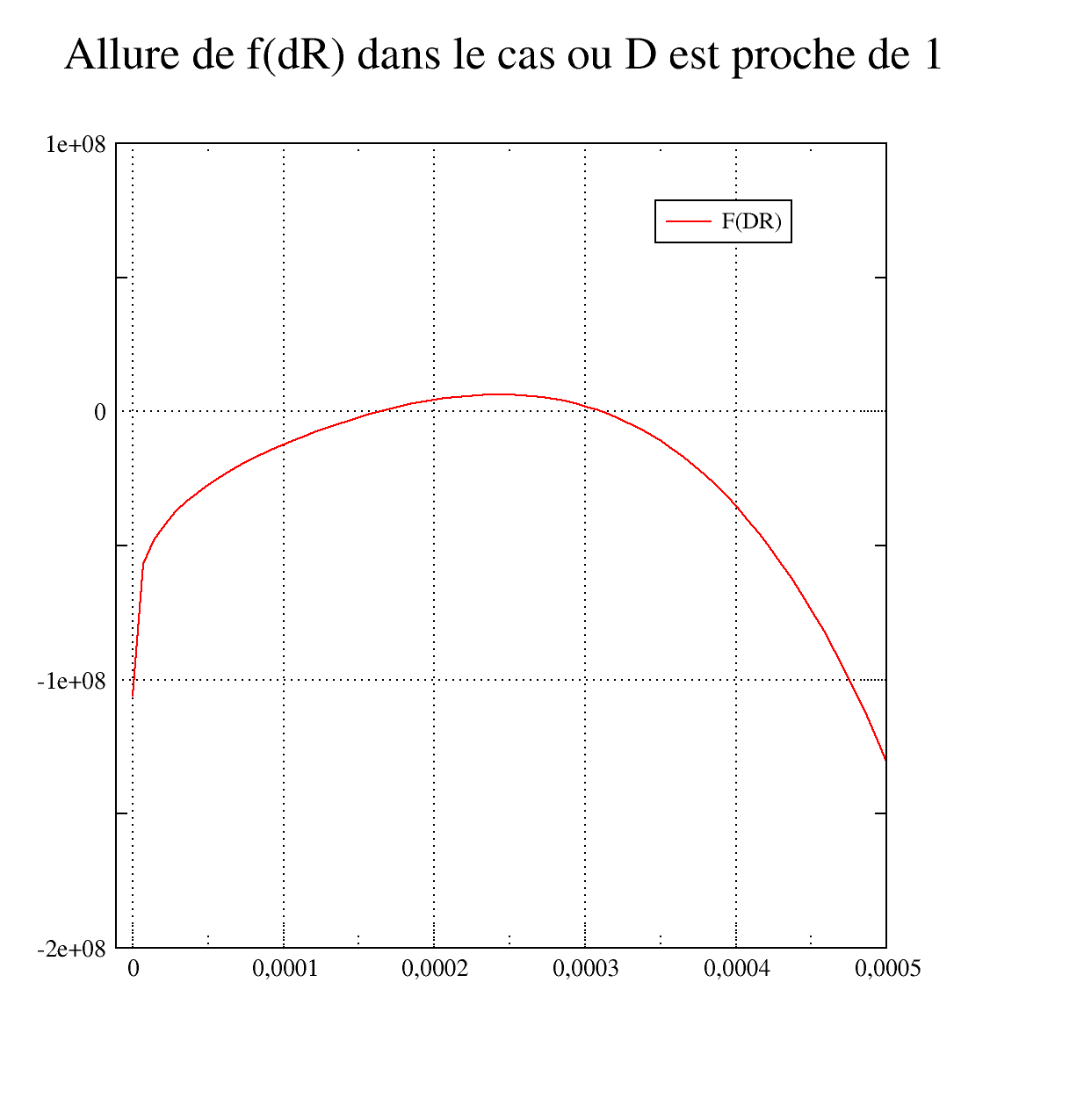
\(\begin{array}{}\Delta r\text{solution de :}\\ f(\Delta r)=(1-D)(K{(\Delta r)}^{1/N}{r}^{1/M}+{\sigma }_{y}{(\Delta t)}^{1/N})+3\mu \Delta r{(\Delta t)}^{1/N}-(1-D){s}^{{e}_{\text{eq}}}{(\Delta t)}^{1/N}=0\end{array}\)

In fact, \(D\) cannot increase to 1, but is limited to \(0.99\), which makes it possible to avoid singular tangent matrices.

To find the solution of this equation, a secant method is used, after obtaining a framework. The function \(f\) is negative in 0 by construction. It’s about looking for an upper bound for which \(f\) is positive.

\(\{\Delta r=-\frac{(1-D)}{3\mu }(K{(\frac{\Delta r}{\Delta t})}^{}{r}^{}+{\sigma }_{y})+\frac{(1-D)}{3\mu }{s}^{{e}_{\text{eq}}}\le \frac{(1-D)}{3\mu }{s}^{{e}_{\text{eq}}}\le \frac{1}{3\mu }{s}^{{e}_{\text{eq}}}\)

If \(f(\frac{1}{3\mu }{s}^{{e}_{\text{eq}}})>0\), then the framework is well defined. The solution is sought within an interval defined by the limits: \([\mathrm{0,}\frac{1}{\mathrm{3\mu }}{s}^{{e}_{\text{eq}}}]\).

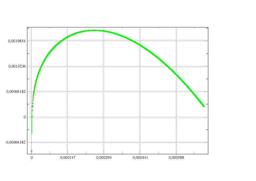
Otherwise, you have to look for an upper bound that makes the function positive. However, this function generally has two solutions: on the following curve the following curve the function \(f(\Delta r)\) is represented in two particular cases: for a situation where \(D\) is small, and for a situation where \(D\) is close to 1. We can see that the function crosses the x-axis twice. The solution we are looking for is the one that corresponds to \(\Delta r\) minimum.

To do this, since \(f(\frac{1}{3\mu }{s}^{{e}_{\text{eq}}})<0\), we calculate the derivative of \(f\). If est is positive we increase the upper bound until we find a value such that \(f\) is positive. If the derivative is negative, we decrease the value of the limit to obtain \(f>0\). The rope method is then applied.

The precision chosen for the resolution is \(\text{RESI\_INTE\_RELA}\ast f(0)\).

Once the value of \(\Delta r\) is obtained, we immediately have that of \(\Delta D\), then the constraint deviator is calculated by:

\({\sigma }^{\text{'}}=(1-D){(1+\frac{3\mu \Delta r}{{\sigma }_{\text{eq}}})}^{-1}{s}^{e}\)

and the trace by:

\(\text{tr}(\Delta \varepsilon -\Delta {\varepsilon }^{\text{th}})+(\frac{\text{tr}{\sigma }^{-}}{{(3\lambda +2\mu )}^{-}(1-{D}^{-})})=\frac{\text{tr}(\sigma )}{(3\lambda +2\mu )(1-D)}\)