6. Use#
These models are accessible in Code_Aster in 3D, plane deformations (D_ PLAN), plane stresses (C_ PLAN, by the De Borst [R5.03.03] method) and axisymmetry (AXIS).
6.1. Single crystal case#
In the case of meshed microstructures, the various grains of a monocrystal being represented by groups of meshes, it is necessary to assign the parameters of the materials and the behaviors of the monocrystals as well as their orientations as well as their orientations to the various grains.
Parameter values for behavioral relationships are provided using the DEFI_MATERIAU command. This is defined using the keywords MONO_VISC1, MONO_VISC2, MONO_DD_KR, MONO_DD_CFC for flow, MONO_ISOT1, MONO_ISOT2, MONO_DD_CFC for isotropic work hardening and MONO_CINE1, MONO_CINE2 for kinematic work hardening [U4.43.01]. For example [V6.04.172]:
MATER1 = DEFI_MATERIAU (

/ELAS =_F (E=..., NU= ... ,

/ELAS_ORTH =_F (E_L=192500,

E_T=128900,

NU_LT =0.23,

G_LT=74520,),


RELATIONS from ECOULEMENT

/MONO_VISC1 =_F (N=10, K=40, C=6333),

/MONO_VISC2 =_F (N=10, K=40, C=6333, D=37, A=121),

/MONO_DD_KR =_F ( ... ),


ECROUISSAGE ISOTROPE

/MONO_ISOT1 =_F (R_0=75.5, Q=9.77, B=19.34, H=2.54),

/MONO_ISOT2 =_F (R_0=75.5, Q1=9.77, B1=19.34, H=2.54, Q2=-33.27, B2=5.345,),


ECROUISSAGE CINEMATIQUE


/MONO_CINE1 =_F (D=36.68),

/MONO_CINE2 =_F (D=36.68, GM=, PM=,),

);
It is thus possible to dissociate, at the data level, the flow from isotropic work hardening and kinematic work hardening.
It is now necessary to define the (or the) type of monocrystal studied. To do this, we define the behavior externally to STAT_NON_LINE, using the DEFI_COMPOR operator, for example:
MONO1 = DEFI_COMPOR (MONOCRISTAL =( _F (MATER = MATER1,
ECOULEMENT = MONO_VISC1,
MONO_ISOT = MONO_ISOT1,
MONO_CINE = MONO_CINE1,
FAMI_SYST_GLIS =( “CUBIQUE1”,),
_F (MATER = MATER1,
ECOULEMENT = MONO_VISC1,
MONO_ISOT = MONO_ISOT2,
MONO_CINE = MONO_CINE2,
FAMI_SYST_GLIS =” CUBIQUE2 “,),
),
_F (MATER = MATER2,
ECOULEMENT = MONO_VISC1,
MONO_ISOT = MONO_ISOT2,
MONO_CINE = MONO_CINE2,
FAMI_SYST_GLIS =” PRISMATIQUE “,),
_F (MATER = MATER2,
ECOULEMENT = MONO_VISC1,
MONO_ISOT = MONO_ISOT2,
MONO_CINE = MONO_CINE2,
FAMI_SYST_GLIS =” BCC24 “,),),
)
The operator DEFI_COMPOR calculates the total number of internal variables associated with the single crystal.
Finally, to perform a micro-structure calculation, it is necessary to give an orientation, grain by grain, or by group of elements (representing sets of grains), using the keyword MASSIF from AFFE_CARA_ELEM. For example:
ORIELEM = AFFE_CARA_ELEM (MODELE = MO_MECA, MASSIF =(

_F (GROUP_MA =' GRAIN1 ', ANGL_REP =( 348.0,24.0,172.0),),

_F (GROUP_MA =' GRAIN2 ', ANGL_REP =( 327.0, 126.0, 335.0),),

_F (GROUP_MA =' GRAIN3 ', ANGL_REP =( 235.0, 7.0, 184.0),),

_F (GROUP_MA =' GRAIN4 ', ANGL_REP =( 72.0, 38.0, 73.0),,

...)
Note 1:
The orientations of the sliding systems can be entered in nautical angles under the keyword ANGL_REPou and Euler angles under the keyword ANGL_EULER.
Note 2:
|
The other calculation data is identical to a usual structural calculation.
Finally, in STAT_NON_LINE, the behavior from DEFI_COMPOR is provided, under the keyword COMPORTEMENT via the keyword COMPOR, mandatory with the keyword RELATION =” MONOCRISTAL “.
COMPORTEMENT = _F (RELATION =' MONOCRISTAL ', COMPOR = COMP1
Note that for explicit integration, (ALGO_INTE =” RUNGE_KUTTA “), it is useless to ask for the tangent matrix to be updated since it is not calculated. To start Newton iterations of the global algorithm, it may be useful to specify PREDICTION =” EXTRAPOLE “[U4.51.03].
Examples of use can be found in the tests: SSNV171, SSNV172, SSNV194.
6.2. Polycrystal case#
In the case of multiphase polycrystals, each phase corresponds to a single crystal. The parameters defined previously in DEFI_MATERIAU for the monocrystal will therefore be used. Here, it is a question of defining, for each phase, the orientation, the volume fraction, the monocrystal used, and the type of localization law. This is done under the keyword factor POLYCRISTAL from DEFI_COMPOR.
MONO1 = DEFI_COMPOR (MONOCRISTAL =_F (MATER = MATPOLY,
ECOULEMENT =” MONO_VISC2 “,
MONO_ISOT =” MONO_ISOT2 “,
MONO_CINE =” MONO_CINE1 “,
ELAS =” ELAS “,
FAMI_SYST_GLIS =” OCTAEDRIQUE “,),);
POLY1 = DEFI_COMPOR (POLYCRISTAL =( _F (MONOCRISTAL = MONO1,
FRAC_VOL =0.025,
ANGL_REP =( -149.676,15.61819,154.676,),),
_F (MONOCRISTAL = MONO1,
FRAC_VOL =0.025,
ANGL_REP =( -150.646,33.864,55.646,),),
_F (MONOCRISTAL = MONO1,
FRAC_VOL =0.025,
ANGL_REP =( -137.138,41.5917,142.138,),),
…
_F (MONOCRISTAL = MONO1,
FRAC_VOL =0.025,
ANGL_REP =( -481.729,35.46958,188.729,),),),
LOCALISATION =” BETA “,
MU_LOCA =80000,,
DL=321.5,
DA=0.216,);
The keyword POLYCRISTAL makes it possible to define each phase by the data of an orientation, (provided by ANGL_REP or ANGL_EULER), of a volume fraction, of a monocrystal (i.e. a behavior model and sliding systems).
The keyword LOCALISATION makes it possible to choose the location method for all the phases of the polycrystal.
The key word MASSIF makes it possible to choose a global orientation of the polycrystal under the keyword ANGL_REP if it is in nautical angles or under the keyword ANGL_EULER if it is in Euler angles.
Finally, in STAT_NON_LINE, the behavior from DEFI_COMPOR is provided, under the keyword COMPORTEMENT via the keyword COMPOR, mandatory with the keyword RELATION =” POLYCRISTAL “.
COMPORTEMENT = _F (RELATION =' POLYCRISTAL ',
COMPOR = COMP1)
6.3. example#
As an example of implementation, an aggregate calculation, of cubic form (elementary volume) comprising 100 monocrystalline grains, each defined by a group of elements, is briefly presented here. The total number of items is 86751. With first order meshes (TETRA4) it has 15940 knots. With 2nd order meshes (TETRA10), it includes 121534.
The load consists of a homogeneous deformation, applied by means of a normal displacement imposed on one face of the cube (direction \(z\)). A deformation of 4% is achieved in 1 s and 50 increments.
ACIER = DEFI_MATERIAU (ELAS =_F (E=145200.0, NU=0.3,),

MONO_VISC1 =_F (N=10., K=40. , C=10.,),

MONO_ISOT2 =_F (R_0=75.5,

B1=19.34,

B2=5.345,

Q1 =9.77,

Q2 =33.27,

H=0.5),

MONO_CINE1 =_F (D=36.68,),);
COEF = DEFI_FONCTION (NOM_PARA =' INST ', VALE =( 0.0,0.0,1.0,1.0,),);

MAT = AFFE_MATERIAU (MAILLAGE = MAIL, AFFE =_F (TOUT =" OUI ", MATER =( ACIER),),);


COMPORT = DEFI_COMPOR (MONOCRISTAL =( _F (MATER = ACIER,

ECOULEMENT =" MONO_VISC1 ",

MONO_ISOT =" MONO_ISOT2 ",

MONO_CINE =" MONO_CINE1 ",

ELAS =" ELAS ",

FAMI_SYST_GLIS =' OCTAEDRIQUE ',),

),);


ORIELEM = AFFE_CARA_ELEM (MODELE = MO_MECA, MASSIF =(

_F (GROUP_MA =' GRAIN1 ', ANGL_REP =( 348.0,24.0,172.0),),

_F (GROUP_MA =' GRAIN2 ', ANGL_REP =( 327.0, 126.0, 335.0),),

_F (GROUP_MA =' GRAIN3 ', ANGL_REP =( 235.0, 7.0, 184.0),),

...

_F (GROUP_MA =' GRAIN99 ', ANGL_REP =( 201.0, 198.0, 247.0),),

_F (GROUP_MA =' GRAIN100 ', ANGL_REP =( 84.0, 349.0, 233.0),),

))


FO_UZ = DEFI_FONCTION (NOM_PARA = 'INST', VALE = (0.0, 0.0, 1.0, 0.04,),)


CHME4 = AFFE_CHAR_MECA_F (MODELE = MO_MECA, DDL_IMPO =_F (GROUP_NO =' HAUT ', DZ= FO_UZ,),)


LINST = DEFI_LIST_REEL (DEBUT = 0. , INTERVALLE =( _F (JUSQU_A = 1. , NOMBRE = 50),))


SIG = STAT_NON_LINE (MODELE = MO_MECA, CARA_ELEM = ORIELEM, CHAM_MATER = MAT,

EXCIT =( _F (CHARGE = CHME1),

_F (CHARGE = CHME2),

_F (CHARGE = CHME3),

_F (CHARGE = CHME4),),

COMPORTEMENT =_F (RELATION =' MONOCRISTAL ', COMPOR = COMPORT),

INCREMENT =_F (LIST_INST = LINST),)
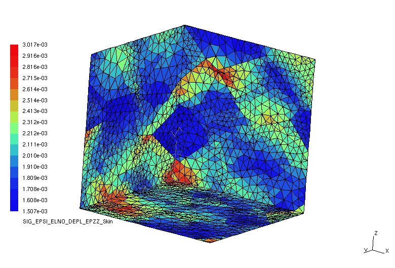
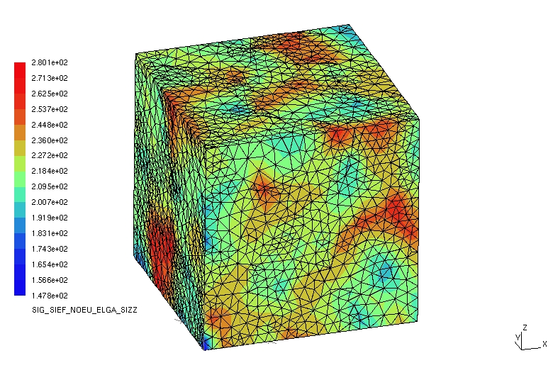
The following figures represent isovalues of the deformations the stresses following \(z\). We note the non-homogeneity of the values, and we can even discern the outline of the grains.
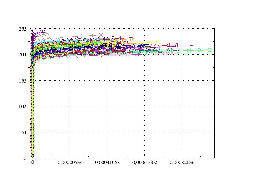
To be able to exploit this type of results, we can for example calculate average fields per grain. In the following figure, the equivalent stresses are represented as a function of the equivalent plastic deformations for all the grains.