2. background

2.1. Problem

We consider the quadratic modal problem (QEP)

Find \((\lambda ,u)\) such as \(({\lambda }^{2}\mathrm{B}+\lambda \mathrm{C}+\mathrm{A})\mathrm{u}\mathrm{=}\mathrm{0,}\mathrm{u}\mathrm{\ne }0\) (2.1-1)

where \(\mathrm{A},\mathrm{B}\) and \(\mathrm{C}\) have square matrices of size \(n\), with real or complex coefficients, symmetric or not. In mechanics, this type of problem corresponds in particular to the study of the free vibrations of a damped and/or rotating structure. For this structure, we look for the eigenvalues \({\lambda }_{i}\) (and their associated eigenvectors \({\mathrm{u}}_{i}\)) that are closest, in the complex plane, to a given reference value (the « shift » \(\sigma\)) to know if an exciting force can create a resonance. In this standard case,

• The matrix \(\mathrm{A}\) is the stiffness matrix, noted \(\mathrm{K}\), real symmetric (possibly increased by the complex symmetric matrix, noted \({\mathrm{E}}_{\mathit{hyst}}\), if the structure has hysteretic damping): \(\mathrm{A}\mathrm{=}\mathrm{K}+{\mathrm{E}}_{\mathit{hyst}}\). So \(\mathrm{A}\) is symmetric real or complex.

• The \(\mathrm{B}\) matrix is the mass or inertia matrix denoted \(\mathrm{M}\) (real symmetric).

The matrix :math:`mathrm{C}` includes possible gyroscopic effects and those of viscous damping*via the combination:

\(\mathrm{C}\mathrm{:}\mathrm{=}{\mathrm{E}}_{\mathit{visq}}+\xi \mathrm{G}\) (2.1-2)

with \({\mathrm{E}}_{\mathrm{visq}}\), a (real symmetric) damping matrix induced by dissipative forces, \(\mathrm{G}\) gyroscopy matrix (real anti-symmetric) and \(\xi\) a real parameter representative of the rotation speed. So \(\mathrm{C}\) is potentially not symmetric real.

This type of problem is activated by the keyword TYPE_RESU =” DYNAMIQUE “. In the general case of QEP (2.1-1) and using only their property of symmetry and matrix arithmetic, we can decompose the perimeter of the Code_Aster modal operators as follows.

\(\mathrm{A}\) / \(\mathrm{C}\)	Symmetric real	Non-symmetric real	Complex
Symmetric real	Most common case SIMULT/INV with no restrictions on methods; Real modes or complexes \((\lambda ,\stackrel{ˉ}{\lambda })\).	SIMULTavec “SORENSEN” /”QZ “; Real or complex modes \((\lambda ,\stackrel{ˉ}{\lambda })\).	Untreated case
Non-symmetric real	SIMULTavec “SORENSEN” /”QZ “; Real modes or complexes \((\lambda ,\stackrel{ˉ}{\lambda })\).	SIMULTavec “SORENSEN” /”QZ “ Real or complex modes \((\lambda ,\stackrel{ˉ}{\lambda })\).	Untreated case
Symmetric complex	SIMULTavec “SORENSEN” /”QZ “ Real, complex, any modes, or \((\lambda ,\stackrel{ˉ}{\lambda })\).	Untreated case	Untreated case
Other complexes (Hermitian, non-symmetric…)	Untreated case	Untreated case	Untreated case	Untreated case

Table 2.1-1. Scope of use of the Aster operator CALC_MODES according to the analysis methods, depending on the properties of the matries \(\mathrm{A}\) and \(\mathrm{C}\) of the QEP (2.1-1) . \(\mathrm{B}\) is any real.

In the absence of hysteretic damping, the QEP standard to be solved therefore consists of symmetric real matrixs. These eigenvalues are either real or complex conjugated in pairs \((\lambda ,\stackrel{ˉ}{\lambda })\). The eigenvectors then potentially have complex components.

In the presence of hysteretic damping, QEP becomes complex and loses the previous property [1] _ . These modes are then real, complex in pairs or mismatched.

Notes:

*Unlike GEP [Boi09] processed by Code_Aster, the keyword TYPE_RESU =” FLAMBEMENT “*is not legal within the framework of QEP. *

• Computatively, the scope of option [“CENTRE”, “PLUS_PETITE”, “”, “TOUT”] has been extended to real non-symmetric matrices \(\mathrm{A},\mathrm{B}\text{et}\mathrm{C}\) of QEP. This is not yet the case for option [“PROCHE”, “AJUSTE”] which is limited, for the moment, to symmetric real matrices. The latter cannot therefore take into account gyroscopic effects.

The damping modeling [Lev96] in Code_Aster can be broken down into two classes: proportional viscous damping (called Rayleigh damping :math:`{mathrm{E}}_{mathit{visq}}mathrm{:}mathrm{=}alpha mathrm{K}+beta mathrm{M}`) or hysteretic damping (:math:`{mathrm{E}}_{mathit{hist}}mathrm{:}mathrm{=}(1+ieta )mathrm{K}`). Each is available at the global level of the structure or by means of localized amortization (groups of cells, ad hoc discrete elements). The latter make it possible to better represent the heterogeneity of the structure in relation to damping. However, there is still the delicate question of identifying the coefficients*:math:`(alpha ,beta eta )`*and their influences on the result. *

2.2. Properties of clean modes

The preceding table 2.2-1 does not take into account particular cases (pure gyroscopy, over-damped structure, etc.). For the record, we will list some of them that are often found in literature. But it should be remembered that the context of Code_Aster models (almost systematic use of double Lagranges) and the sorting of eigenmodes programmed in modal operators do not take these specificities into account. Currently in QEP, we only retain coupled modes \((\lambda ,\stackrel{ˉ}{\lambda })\) and we keep the one with a positive imaginary part. Depending on the case, the presence of eigenvalues of other types (real or complex non-conjugated) is indicated by a ALARME or for information purposes.

We therefore have (using the elements and the notations from §3.3 of [Boi09] and the paper [TM01]), we have the distribution of the following properties. These are sometimes cumulative. Figures 2.2-1 and 2.2-2 illustrate, on canonical cases, some cases.

Table 2.2-1. Properties of the modes of a standard QEP (of size \(n\) ) according to those of its matrices. Possible links with Code_Aster models.

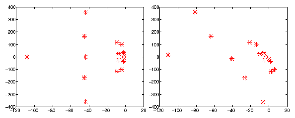
Figure 2.2-1. Examples of the spectrum of a QEP \((n=8)\) of a simplified nuclear enclosure model [TM01]. Figure on the left, we are in case No. 3 of table 2.2-1. The one on the right, we add hysteretic damping to \(\mathrm{K}\) so mismatched modes appear (general case no. 1) .

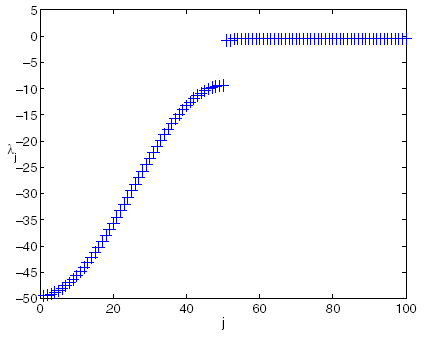
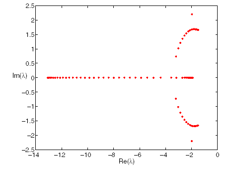
Figure 2.2-2. Examples of the spectrum of a QEP \((n=50)\) of a damped mass-spring system [TM01]. Figure on the left, we are in case No. 5 of table 2.2-1. The one on the right, we add the over-damping constraint and the spectrum becomes real negative in two packets (case no. 6).

2.3. Specificities of QEP and elements of theory

A major algebraic specificity between QEP and the other lower-level modal problem classes (GEP and SEP) is the existence of twice as many eigenmodes ( \(\mathrm{2n}\) ) as the size of the discretized problem. Eigenvectors can no longer be linearly independent, in addition, eigenvalues can be finite or infinite and all « this little world » generally lives in the complex plane [3] _ . It is then necessary define robust heuristics to filter the eigenvalues desired by the user and distinguish the real ones, the complex ones, the mismatched complexes from the coupled ones…

Another complication inherent in QEP is algorithmic. There is no Schur decomposition (or generalized Schur) as for SEP (resp. GEP) on which the resolution algorithm will be able to rely. For example, for SEP \(\mathrm{A}\mathrm{u}\mathrm{=}\lambda \mathrm{u}\), this decomposition assures us of the existence of a unitary matrix (therefore well-conditioned and easily invertible) \(\mathrm{U}\), allowing the rewriting of the working matrix \(\mathrm{A}\) in a form that is easier to handle [4] _ : the upper triangular matrix \(\mathrm{T}\).

\(\mathrm{U}\mathrm{A}{\mathrm{U}}^{\text{*}}\mathrm{=}\mathrm{T}\) (2.3-1)

The QEP are therefore a very particular and important class [5] _ nonlinear problems. Solving them is less routine than for other classes of modal problems. In particular, few methods make it possible to solve the problem directly, it is often necessary to go through a GEP (via a *ad hoc linearization) then a SEP (spectral transformation) which induces a loss of spectral information and numerical instabilities (propagation of rounding errors).

In theoretical literature, rather than QEP (2.1-1), we are interested in the matrix polynomial (quadratic in \(\lambda\))

\(\mathrm{Q}(\lambda )\mathrm{:}\mathrm{=}({\lambda }^{2}\mathrm{B}+\lambda \mathrm{C}+\mathrm{A})\) (2.3-2)

We also call it \(\lambda \text{-matrice}\) or dynamic matrix and we are looking for its spectrum denoted \(\mathit{spectre}(\mathrm{Q})\mathrm{:}\mathrm{=}\mathrm{\{}\lambda \mathrm{\in }C\mathrm{/}\mathit{det}\mathrm{Q}(\lambda )\mathrm{=}0\mathrm{\}}\). When this determinant is zero regardless of \(\lambda\), \(\lambda \text{-matrice}\) is said to be singular. Otherwise, it is said to be regular (we generally place ourselves in this framework!).

The characteristic polynomial of the problem is therefore written in the form \(\mathit{det}\mathrm{Q}(\lambda )\mathrm{=}\mathit{det}(\mathrm{B}){\lambda }^{\mathrm{2n}}+\) lower-order terms in \(\lambda\). Thus, as soon as \(\mathrm{B}\mathrm{=}\mathrm{M}\) is singular, this polynomial admits \(r<\mathrm{2n}\) finite roots to which must be added \(\mathrm{2n}-r\) infinite. On the other hand, these distinct eigenvalues can share the same eigenvectors. This is the « dual situation » of multiple eigenvalues in SEP where the same eigenvalue is attached to several eigenvectors. So for the canonical QEP

\(\mathrm{A}\mathrm{=}{\mathrm{I}}_{\mathrm{3,}}\mathrm{B}\mathrm{=}\left[\begin{array}{ccc}0& 6& 0\\ 0& 6& 0\\ 0& 0& 1\end{array}\right]\text{et}C\mathrm{=}\left[\begin{array}{ccc}1& \mathrm{-}6& 0\\ 2& \mathrm{-}7& 0\\ 0& 0& 0\end{array}\right]\) (2.3-3)

We have the following spectrum

\(\begin{array}{ccccccc}i& 1& 2& 3& 4& 5& 6\\ {\lambda }_{i}& 1\mathrm{/}3& 1\mathrm{/}2& 1& i& \mathrm{-}i& \mathrm{\infty }\\ {\mathrm{u}}_{i}& \left[\begin{array}{c}1\\ 1\\ 0\end{array}\right]& \left[\begin{array}{c}1\\ 1\\ 0\end{array}\right]& \left[\begin{array}{c}0\\ 1\\ 0\end{array}\right]& \left[\begin{array}{c}0\\ 0\\ 1\end{array}\right]& \left[\begin{array}{c}0\\ 0\\ 1\end{array}\right]& \left[\begin{array}{c}1\\ 0\\ 0\end{array}\right]\end{array}\) (2.3-4)

From the uniqueness of \(\mathrm{B}\) comes the infinite eigenvalue. We also note the sharing of eigenvectors by the first two eigenvalues and the 4th/5th.

To more easily understand the infinite eigenvalues of \(\mathrm{Q}(\lambda )\), we associate them with the zero eigenvalues of the inverse polynomial

\(\mathit{rev}\mathrm{Q}(\lambda )\mathrm{:}\mathrm{=}{\lambda }^{2}\mathrm{Q}(\frac{1}{\lambda })\mathrm{=}(\mathrm{B}+\lambda \mathrm{C}+{\lambda }^{2}\mathrm{A})\) (2.3-5)

These finite eigenvalues of \(\mathit{rev}\mathrm{Q}(\lambda )\) are easier to calculate and share the same spectral characteristics (geometric and algebraic multiplicities, eigenspace…) as the initial infinite values.

For more information on these theoretical aspects one can consult, for example, the works of P.Lancaster [GLR82] [LT85] and the thesis of D.S.Mackey [Mac06] (and its numerous bibliographical references).

2.4. Linearization strategy

2.4.1. Introduction

The standard approach to solving a modal problem is to transform it to reveal canonical matrices revealing the modes sought. For example, the Schur decomposition for SEP or the generalized one for GEP. Unfortunately, this practice cannot be generalized to higher-order modal problems. Two solutions are then available:

• Solve the non-linear problem directly (polynomial root, factorization of \(\lambda \text{-matrice}\), Newtons-type methods…).

• Linearize it into a GEP, then process it via using the appropriate methods [Boi09].

The first strategy is available in the options [“PROCHE”, “AJUSTE”] (Müller-Traub method) to capture a first estimate of eigenvalues. We then mix it up with the following strategy, because to refine the estimates and accelerate convergence, we use an inverse power method (Jennings variant) on the linearized QEP. Some authors offer comprehensive direct approaches. They are often based on Newton’s variants. But their convergence is slow (one mode at a time) and not always assured (cf. Kublanovskaya 1970, G.Peters & J.H.Wilkinson 1979 and A.Ruhe 1973).

The linearization strategy is therefore often preferred. It doubles the size of the modal problem to be treated, changes its nature (at the risk of losing spectral information) [6] _ ) and introduces numerical instabilities (sensitivity to rounding errors [7] _ and to the numerical parameters [8] _ ). But it has the immense advantage of reusing all the « digital artillery » already deployed for the GEP [9] _ .

It is thus possible to simultaneously capture the entire spectrum (cf. the QZ method usable with the options [“CENTRE”, “PLUS_PETITE”, “TOUT”]) or only the part centered on an area of interest (cf. IRAM or Lanczos) using the appropriate spectral transformation.

2.4.2. Principle

Now that the context has been outlined, to conform to the terminology used in the literature, we will now simplify the notations by considering the QEP associated with the \(\lambda \text{-matrice}\) \(\mathrm{Q}(\lambda )\mathrm{:}\mathrm{=}({\lambda }^{2}\mathrm{M}+\lambda \mathrm{C}+\mathrm{K})\). This matrix is also called a « dynamic matrix » in structural dynamics jargon (and in Code_Aster computer documents/sources). It is the counterpart to the one described in the note dedicated to GEP: \(\mathrm{Q}(\lambda )\mathrm{:}\mathrm{=}(\mathrm{K}\mathrm{-}\lambda \mathrm{M})\).

Definition 1

From a theoretical point of view, linearizing \(\mathrm{Q}(\lambda )\) is the same as finding another \(\lambda \text{-matrice}\) (square complex of size \(\mathrm{2n}\)) of the type \(\mathrm{A}\mathrm{-}\lambda \mathrm{B}\) such that there are two other \(\lambda \text{-matrices}\) (\(\mathrm{E}(\lambda )\) and \(\mathrm{F}(\lambda )\)) with a non-zero constant determinant, verifying the relationship

\(\left[\begin{array}{cc}\mathrm{Q}(\lambda )& {0}_{n}\\ {0}_{n}& {\mathrm{I}}_{n}\end{array}\right]\mathrm{=}\mathrm{E}(\lambda )(\mathrm{A}\mathrm{-}\lambda \mathrm{B})\mathrm{F}(\lambda )\) (2.4-1)

The matrices \(\mathrm{A}\) and \(\mathrm{B}\) are called the « companion » matrices for the linearization of QEP.

Clearly, the spectra of the initial QEP \((\mathrm{Q}(\lambda ))\) and that of its linearization \((\mathrm{A}\mathrm{-}\lambda \mathrm{B})\) coincide. However this decomposition is not unique and it is necessary to choose, if possible, the one that:

• Preserves the properties of the initial matrices (arithmetic, symmetry…),

Has the**least sensitivity to rounding errors* (« stable backward »: balanced, well-conditioned, invertible matrices…),

Manipulates**canonical matrix* (identity, triangular…),

Adapts to a**large perimeter of QEP * (viscous damping, gyroscopic, over-damping…).

A more intuitive way to understand linearization techniques is to introduce a variable change of the type \(\mathrm{v}\mathrm{=}\lambda \mathrm{u}\) [10] _ in (2.1-1) and rearranging it in matrix form:

\((\underset{\mathrm{A}}{\underset{\underbrace{}}{\left[\begin{array}{cc}{0}_{n}& {\mathrm{I}}_{n}\\ \mathrm{-}\mathrm{K}& \mathrm{-}\mathrm{C}\end{array}\right]}}\mathrm{-}\lambda \underset{\mathrm{B}}{\underset{\underbrace{}}{\left[\begin{array}{cc}{\mathrm{I}}_{n}& {0}_{n}\\ {0}_{n}& \mathrm{M}\end{array}\right]}})\left[\begin{array}{c}\mathrm{u}\\ \mathrm{v}\end{array}\right]\mathrm{=}{0}_{\mathrm{2n}}\) (2.4-2)

This « very classical » linearization falls within the framework of definition 1 if we use \(\lambda \text{-matrices}\):

\(\mathrm{E}(\lambda )\mathrm{:}\mathrm{=}\left[\begin{array}{cc}\mathrm{-}(\mathrm{C}+\lambda \mathrm{M})& \mathrm{-}{\mathrm{I}}_{n}\\ {\mathrm{I}}_{n}& {0}_{n}\end{array}\right],\mathrm{F}(\lambda )\mathrm{:}\mathrm{=}\left[\begin{array}{cc}{\mathrm{I}}_{n}& {0}_{n}\\ \lambda {\mathrm{I}}_{n}& {\mathrm{I}}_{n}\end{array}\right]\) (2.4-3)

In fact, the linearization of a QEP follows the general framework of that of matrix polynomials. By setting \(\mathrm{Q}(\lambda )\mathrm{:}\mathrm{=}\mathrm{\sum }_{i\mathrm{=}1}^{k}{\lambda }_{i}{\mathrm{X}}_{i}\) (here \(k\mathrm{=}\mathrm{2,}{\mathrm{X}}_{i}\mathrm{=}\mathrm{M}\) etc), we are always sure to find two linearizations, called « companions », of the form \({\mathrm{A}}_{1}\mathrm{-}\lambda {\mathrm{B}}_{1}\) and \({A}_{2}-\lambda {B}_{2}\) with

\(\begin{array}{cc}{\mathrm{B}}_{1}\mathrm{=}{\mathrm{B}}_{2}\mathrm{:}\mathrm{=}\left[\begin{array}{cc}\mathrm{-}{\mathrm{X}}_{k}& {0}_{(k\mathrm{-}1)n}\\ {0}_{(k\mathrm{-}1)n}& \mathrm{-}{\mathrm{I}}_{(k\mathrm{-}1)n}\end{array}\right],& \\ {\mathrm{A}}_{1}\mathrm{:}\mathrm{=}\left[\begin{array}{cccc}{\mathrm{X}}_{k\mathrm{-}1}& {\mathrm{X}}_{k\mathrm{-}2}& \text{...}& {\mathrm{X}}_{0}\\ {\mathrm{I}}_{n}& {0}_{n}& \text{...}& {0}_{n}\\ \text{...}& \text{...}& \text{...}& \text{...}\\ {0}_{n}& \text{...}& \mathrm{-}{\mathrm{I}}_{n}& {0}_{n}\end{array}\right],& {\mathrm{A}}_{2}\mathrm{:}\mathrm{=}\left[\begin{array}{cccc}{\mathrm{X}}_{k\mathrm{-}1}& \mathrm{-}{\mathrm{I}}_{n}& \text{...}& {0}_{n}\\ {\mathrm{X}}_{k\mathrm{-}2}& {0}_{n}& \text{...}& \text{...}\\ \text{...}& \text{...}& \text{...}& \mathrm{-}{\mathrm{I}}_{n}\\ {\mathrm{X}}_{0}& {0}_{n}& \text{...}& {0}_{n}\end{array}\right]\end{array}\) (2.4-4)

In practice, linearizations that are more adapted to the case being treated are preferred (cf. next paragraph).

2.4.3. A few examples

In the literature, the following linearizations** are often mentioned (with \(N\) a complex regular square matrix of size \(n\)):

(\({L}_{1}\)) \((\underset{\mathrm{A}}{\underset{\underbrace{}}{\left[\begin{array}{cc}{0}_{n}& \mathrm{N}\\ \mathrm{-}\mathrm{K}& \mathrm{-}\mathrm{C}\end{array}\right]}}\mathrm{-}\lambda \underset{\mathrm{B}}{\underset{\underbrace{}}{\left[\begin{array}{cc}\mathrm{N}& {0}_{n}\\ {0}_{n}& \mathrm{M}\end{array}\right]}})\left[\begin{array}{c}\mathrm{u}\\ \lambda \mathrm{u}\end{array}\right]\mathrm{=}{0}_{\mathrm{2n}}\) (2.4-5)

(\({L}_{2}\)) \((\underset{\mathrm{A}}{\underset{\underbrace{}}{\left[\begin{array}{cc}\mathrm{-}\mathrm{K}& {0}_{n}\\ {0}_{n}& \mathrm{N}\end{array}\right]}}\mathrm{-}\lambda \underset{\mathrm{B}}{\underset{\underbrace{}}{\left[\begin{array}{cc}\mathrm{C}& \mathrm{M}\\ \mathrm{N}& {0}_{n}\end{array}\right]}})\left[\begin{array}{c}\mathrm{u}\\ \lambda \mathrm{u}\end{array}\right]\mathrm{=}{0}_{\mathrm{2n}}\) (2.4-6)

The choice depends on the potential singularity of matrices \(\mathrm{K}\) and \(\mathrm{M}\). We want to be able to invert the diagonal terms, so if \(\mathrm{K}\) is singular (resp. \(\mathrm{M}\)), we use (\({L}_{1}\)) (resp. (\({L}_{2}\))). To balance the terms of the matrices and facilitate the manipulations, we often take \(\mathrm{N}\mathrm{=}\alpha {\mathrm{I}}_{n}\) with \(\alpha\) real balancing factor (cf. [Boi09] annex 1) constructed from the matrix norms of the other terms \(\alpha \mathrm{=}\alpha (\mathrm{\parallel }\mathrm{K}\mathrm{\parallel },\mathrm{\parallel }\mathrm{M}\mathrm{\parallel },\mathrm{\parallel }\mathrm{C}\mathrm{\parallel })\). To work with a symmetric GEP (or even positive definite or semi-definite), you can also initialize the auxiliary matrix \(\mathrm{N}\text{à}\alpha \mathrm{K}\text{ou}\beta \mathrm{M}(\alpha ,\beta \mathrm{\in }\mathrm{\Re })\).

To solve QEP with gyroscopic effects more effectively, the literature recommends the « Hamiltonian » counterparts [11] _ «  previous linearizations. Let the « companion » matrices be

(\({L}_{3}\)) \((\underset{\mathrm{A}}{\underset{\underbrace{}}{\left[\begin{array}{cc}\mathrm{K}& {0}_{n}\\ \mathrm{C}& \mathrm{N}\end{array}\right]}}\mathrm{-}\lambda \underset{\mathrm{B}}{\underset{\underbrace{}}{\left[\begin{array}{cc}{0}_{n}& \mathrm{K}\\ \mathrm{-}\mathrm{M}& {0}_{n}\end{array}\right]}})\left[\begin{array}{c}\mathrm{u}\\ \lambda \mathrm{u}\end{array}\right]\mathrm{=}{0}_{\mathrm{2n}}\) (2.4-7)

(\({L}_{4}\)) \((\underset{\mathrm{A}}{\underset{\underbrace{}}{\left[\begin{array}{cc}{0}_{n}& \mathrm{-}\mathrm{K}\\ \mathrm{M}& \mathrm{N}\end{array}\right]}}\mathrm{-}\lambda \underset{\mathrm{B}}{\underset{\underbrace{}}{\left[\begin{array}{cc}\mathrm{M}& \mathrm{C}\\ {0}_{n}& \mathrm{M}\end{array}\right]}})\left[\begin{array}{c}\mathrm{u}\\ \lambda \mathrm{u}\end{array}\right]\mathrm{=}{0}_{\mathrm{2n}}\) (2.4-8)

Here the objective is not to respect a property of symmetry but rather those « Hamiltonian » [12] _ «  of the problem. If \(\mathrm{K}\) is singular (resp. \(\mathrm{M}\)), we use (\({L}_{4}\)) (resp. (\({L}_{3}\))).

In the case of a QEP called « T-palindromic » [Mac06] \((\mathrm{K}\mathrm{=}{\mathrm{M}}^{T}\text{et}\mathrm{C}\mathrm{=}{\mathrm{C}}^{T})\) we prefer linearization

(\({L}_{5}\)) \((\underset{\mathrm{A}}{\underset{\underbrace{}}{\left[\begin{array}{cc}\mathrm{K}& \mathrm{K}\\ \mathrm{C}\mathrm{-}\mathrm{M}& \mathrm{K}\end{array}\right]}}\mathrm{-}\lambda \underset{\mathrm{B}}{\underset{\underbrace{}}{\left[\begin{array}{cc}\mathrm{-}\mathrm{M}& \mathrm{K}\mathrm{-}\mathrm{C}\\ \mathrm{-}\mathrm{M}& \mathrm{-}\mathrm{M}\end{array}\right]}})\left[\begin{array}{c}\mathrm{u}\\ \lambda \mathrm{u}\end{array}\right]\mathrm{=}{0}_{\mathrm{2n}}\) (2.4-9)

2.4.4. Strategies selected in Code_Aster

We therefore have a very wide variety of choices to adapt the linearization of QEP to each situation. For the moment, Code_Aster does not offer the user a parameter that allows the user to modulate only the linearization. This is fixed for a given modal solver:

• With OPTIONparmi [“PROCHE”, “”, “AJUSTE”] (2ndphase) (2ndphase) the transition QEP/GEP is carried out*via*the companion matrices of (L1), by asking :math:`mathrm{N}mathrm{=}{mathrm{I}}_{n}mathrm{.}` The linearized system is not symmetric but it is not a prerequisite for**applying an inverse power method.

(L1) “\((\underset{\mathrm{A}}{\underset{\underbrace{}}{\left[\begin{array}{cc}{0}_{n}& {\mathrm{I}}_{n}\\ \mathrm{-}\mathrm{K}& \mathrm{-}\mathrm{C}\end{array}\right]}}\mathrm{-}\lambda \underset{\mathrm{B}}{\underset{\underbrace{}}{\left[\begin{array}{cc}{\mathrm{I}}_{n}& {0}_{n}\\ {0}_{n}& \mathrm{M}\end{array}\right]}})\left[\begin{array}{c}\mathrm{u}\\ \lambda \mathrm{u}\end{array}\right]\mathrm{=}{0}_{\mathrm{2n}}\) (2.4-10)

• With OPTIONparmi [“CENTRE”, “”, “PLUS_PETITE”] and METHODE =” TRI_DIAG “or “SORENSEN “, the passage QEP/GEP is carried out via the companion matrices of (L2) by setting \(\mathrm{N}\mathrm{=}\mathrm{M}\). If the stiffness, mass and damping matrices are real symmetric, we fall back into the perimeter of the standard GEP (real symmetric). The methods of Lanczos and Sorensen are then accessible. If \(\mathrm{K}\) becomes complex or if one of them is not symmetric, only IRAM remains in the race (with QZ see next item)!

(L2) “\((\underset{\mathrm{A}}{\underset{\underbrace{}}{\left[\begin{array}{cc}\mathrm{-}\mathrm{K}& {0}_{n}\\ {0}_{n}& \mathrm{M}\end{array}\right]}}\mathrm{-}\lambda \underset{\mathrm{B}}{\underset{\underbrace{}}{\left[\begin{array}{cc}\mathrm{C}& \mathrm{M}\\ \mathrm{M}& {0}_{n}\end{array}\right]}})\left[\begin{array}{c}\mathrm{u}\\ \lambda \mathrm{u}\end{array}\right]\mathrm{=}{0}_{\mathrm{2n}}\) (2.4-11)

However, when \(\mathrm{M}\) is not invertable (due to blocking Lagranges for example), the inversion of the diagonal term of \(\mathrm{A}\) is no longer assured. To overcome this problem, a « regularization » of the matrix \(\mathrm{M}\), noted \({M}_{R}\), is introduced into the diagonal term. This has the property of cancelling, by multiplication, all the components of the core of \(\mathrm{M}\mathrm{:}{\mathrm{M}}_{R}\mathrm{u}\mathrm{=}0\text{si}\mathrm{u}\mathrm{\in }\mathit{Ker}(\mathrm{M})\). Thus, we can define \({\mathrm{M}}_{R}^{\mathrm{-}1}\) which formally verifies the \({\mathrm{M}}_{R}^{\mathrm{-}1}\mathrm{M}\mathrm{\approx }\mathrm{M}{\mathrm{M}}_{R}^{\mathrm{-}1}\mathrm{\approx }{\mathrm{I}}_{n}\) property on the « non-core components of \(\mathrm{M}\) » of the manipulated vectors. Because of the particular structure of the dualized matrix \(\mathrm{M}\) (cf. [Boi09] §3.2), this manipulation amounts to proscribing components related to Lagranges and blocked degrees of freedom (the \({\mathrm{v}}_{i}^{\mathrm{2,3}}\) of the demonstration of property no. 4 [Boi09]). This does not hinder the process since we are only interested in physical modes and not in these modeling artifacts [13] _ .

(L2) » \((\underset{\mathrm{A}}{\underset{\underbrace{}}{\left[\begin{array}{cc}\mathrm{-}\mathrm{K}& {0}_{n}\\ {0}_{n}& {\mathrm{M}}_{R}\end{array}\right]}}\mathrm{-}\lambda \underset{\mathrm{B}}{\underset{\underbrace{}}{\left[\begin{array}{cc}\mathrm{C}& \mathrm{M}\\ \mathrm{M}& {0}_{n}\end{array}\right]}})\left[\begin{array}{c}\mathrm{u}\\ \lambda \mathrm{u}\end{array}\right]\mathrm{=}{0}_{\mathrm{2n}}\) (2.4-12)

• With OPTIONparmi [“CENTRE”, “”, “PLUS_PETITE”, “TOUT”] and METHODE =”QZ”,* we preferred to avoid these complications. The objective is to **emphasize numerical robustness to deal with small cases (\(<{10}^{3}\) degrees of freedom). The scenario (L2) was empirically selected by posing \(\mathrm{N}\mathrm{=}\alpha {\mathrm{I}}_{n}\), with, \(\alpha \mathrm{:}\mathrm{=}\frac{1}{\mathrm{3n}}(\mathrm{\parallel }\mathrm{K}\mathrm{\parallel }+\mathrm{\parallel }\mathrm{M}\mathrm{\parallel }+\mathrm{\parallel }\mathrm{C}\mathrm{\parallel })\)

(L2) * \((\underset{\mathrm{A}}{\underset{\underbrace{}}{\left[\begin{array}{cc}\mathrm{-}\mathrm{K}& {0}_{n}\\ {0}_{n}& \alpha {\mathrm{I}}_{n}\end{array}\right]}}\mathrm{-}\lambda \underset{\mathrm{B}}{\underset{\underbrace{}}{\left[\begin{array}{cc}\mathrm{C}& \mathrm{M}\\ \alpha {\mathrm{I}}_{n}& {0}_{n}\end{array}\right]}})\left[\begin{array}{c}\mathrm{u}\\ \lambda \mathrm{u}\end{array}\right]\mathrm{=}{0}_{\mathrm{2n}}\) (2.4-13)

2.5. Implementation in Code_Aster

By design, the process of a quadratic modal calculation is very similar to that of a generalized problem. We will therefore refer to the functional diagram for solving GEP described in [Boi09] (cf. §3.8). Its stages are broken down as follows:

2.5.1. Pre-treatments (linearization, shift calculation)

Determination of the linearized form and the associated spectral transformation according to the method selected (power, Lanczos, IRAM and QZ) and the search option “AJUSTE”/”PROCHE” or “PLUS_PETITE”/”CENTRE”.

Note that since the natural modes are in the complex plane, the Sturm test currently implemented is inoperative. So the heuristic associated with OPTION “PROCHE” and “AJUSTE” is not based on modal positions, and the “BANDE” option is forbidden. Likewise for post-verification based on the Sturm test [Boi12].

For the subspace method (OPTION among [“CENTRE”, “”, “PLUS_PETITE”] and METHODE =” TRI_DIAG “or” SORENSEN “), once the linearized problem \(({L}_{2})’’\) is updated, a « shift-and-invert » spectral transformation is applied (cf. [Boi09] §3.6/§5). This will allow us to complete the transformation into a SEP [14] _ \(({S}_{1})\), to direct the search for the spectrum in an area of interest to the user and to better separate the eigenvalues.

\(({S}_{1})\) \(\underset{{\mathrm{A}}_{\sigma }}{\underset{\underbrace{}}{{(\mathrm{A}\mathrm{-}\sigma \mathrm{B})}^{\mathrm{-}1}}}\mathrm{B}\underset{\mathrm{W}}{\underset{\underbrace{}}{\left[\begin{array}{c}\mathrm{u}\\ \lambda \mathrm{u}\end{array}\right]}}\mathrm{=}\underset{\mu }{\underset{\underbrace{}}{\frac{1}{\lambda \mathrm{-}\sigma }}}\underset{\mathrm{W}}{\underset{\underbrace{}}{\left[\begin{array}{c}\mathrm{u}\\ \lambda \mathrm{u}\end{array}\right]}}\) (2.5-1)

Does the inverse power method apply a specific spectral transformation to the linearized problem \(({L}_{1})’\).

As for the QZ method (OPTION among [“CENTRE”, “”, “PLUS_PETITE”, “TOUT”] and METHODE =”QZ”), this spectral transformation is superfluous. The algorithm directly treats the linearized problem \({({L}_{2})}^{\text{*}}\) and calculates all of its modes. Depending on the user’s wishes (OPTION, CALC_FREQ =_F (NMAX_FREQ…)), it then filters the results.

Notes:

• As with linearization techniques, no user parameter yet allows changing spectral transformations. In quadratic, it would be interesting to use transformations that are more adapted to the complex plane than the traditional « shift-and-invert ». For example, a Cayley transformation to make conjugate eigenvalue pairs converge \((\lambda ,\stackrel{ˉ}{\lambda })\) simultaneously

\(\underset{{\mathrm{A}}_{\sigma }}{\underset{\underbrace{}}{(\mathrm{A}\mathrm{-}\sigma \mathrm{B}){\mathrm{B}}^{\mathrm{-}1}(\mathrm{A}\mathrm{-}\stackrel{ˉ}{\sigma }\mathrm{B}){\mathrm{B}}^{\mathrm{-}1}}}\mathrm{w}\mathrm{=}\underset{\mu }{\underset{\underbrace{}}{\frac{1}{(\lambda \mathrm{-}\sigma )(\stackrel{ˉ}{\lambda }\mathrm{-}\sigma )}}}\mathrm{W}\) (2.5-2)

• This Cayley strategy is being generalized to treat gyroscopy (see V.Mehrman and D.Watkins 2001) and simultaneously converge quadruplets \((\lambda ,\stackrel{ˉ}{\lambda },-\lambda ,-\stackrel{ˉ}{\lambda })\)

• Some authors also propose to invert the linearization phase and the spectral transformation phase [Mee07].

2.5.2. Factorization of dynamic matrices

As already pointed out, these dynamic matrix factorizations like \(\mathrm{Q}(\lambda )\) are not used to implement a Sturm test. The latter being illegal for QEP. However, they remain a very present and very expensive ingredient [15] _ for:

• Estimate the cost function of the heuristic part (Müller-Traub method) with OPTION =” AJUSTE “.

• When you need to manipulate a work matrix with inverses. To be more effective, we then look for a formulation that only involves \(\mathrm{Q}{(\lambda )}^{\mathrm{-}1}\) (OPTION among [“PROCHE”, “AJUSTE”] + SOLVEUR_MODAL =_F (OPTION_INV +” DIRECT “), or else OPTION among [” CENTRE “,” “,” « ”,” PLUS_PETITE “] + =_F (SOLVEUR_MODAL METHODE =” TRI_DIAG “/” SORENSEN “)).

The global approach (OPTION among [“CENTRE”, “PLUS_PETITE”, “”, “TOUT”] + SOLVEUR_MODAL =_F (METHODE =”QZ”)) is not concerned with this preliminary factorization of the dynamic matrix.

2.5.3. Modal calculation

The modal calculation itself is done: we solve the standard problem SEP, we go back to the intermediate GEP, then to the initial QEP. For each of these conversions, the results of the previous calculation are filtered and transcribed. Regarding eigenvalues (cf. §2.1/2.2) we only remember \(\lambda\) with a positive imaginary part of coupled modes \((\lambda ,\stackrel{ˉ}{\lambda })\mathrm{.}\)

your problem is highly amortized.

real own value (s): 2

complex eigenvalue (s) with conjugate: 107

complex eigenvalue (s) without conjugates: 0

Example 1. Impressions in the alarm message file summarizing the number of modes not retained (here 2 real ones). Excerpt from the sdll123a test case.

For eigenvectors, two possibilities remain open:

• Take directly the first \(n\) components of \(w\) (the so-called « high » part),

• Choose the last \(n\) (so-called « low » part) possibly divided by the same scalar.

In Code_Aster, the second option was selected. This choice is not always trivial [16] _ especially with regard to the quality of the modes and their sensitivity to rounding errors.

With OPTION among [“PROCHE”, “AJUSTE”], only one method is available, a variant of the inverse iteration method due to Jennings (OPTION_INV =” DIRECT “). It refines the eigenvalues previously detected by the Müller-Traub method (“AJUSTE”) or the estimates provided by the user (“PROCHE”). For OPTION among [“CENTRE”, “PLUS_PETITE”, “”, “TOUT”], three distinct methods can be used: the Lanczos method (“TRI_DIAG “), the Sorensen method (” SORENSEN “), and QZ (” QZ “). Only the last two are available with real or complex symmetric non-symmetric matrices (for \(\mathrm{K}\) only).

Remarks

• Each of these methods has internal stop tests. Not to mention that the projection methods use auxiliary modal methods: \(\mathrm{QR}\mathrm{/}\mathrm{QL}\) for Lanczos and IRAM. They also require stop tests. The user often has access to these settings, although it is highly recommended, at least initially, to keep their values by default.

• Unlike GEP, we don’t force the \(\mathrm{M}\) -orthonormalization of eigenvectors. It makes no sense in QEP. Furthermore, applying the result of Proposition 2 of [Boi09] to the linearized problem, it is clear that the eigenvectors are \(\mathrm{A}\) and \(B\) -orthogonal. But due to the complexity of the linear reductions used, this does not lead (except in special cases) to eigenvectors \(\mathrm{K}\) , \(\mathrm{M}\) or \(\mathrm{C}\) -orthogonal!

2.5.4. Audit post-treatments

This last part includes the only post-processing that verifies the smooth running of the calculation (in the absence of a Sturm test adapted to the complex case). We calculate the relative error on the norm [17] _ from the initial QEP residual

\(\begin{array}{c}\mathrm{u}\mathrm{\Leftarrow }\frac{\mathrm{u}}{{〚\mathrm{u}〛}_{\mathrm{\infty }}}\\ \text{Si}\mathrm{\mid }\lambda \mathrm{\mid }>\text{SEUIL\_FREQ}\text{alors}\\ \frac{{∥{\lambda }^{2}\mathrm{Mu}+\lambda \mathrm{Cu}+\mathrm{Ku}∥}_{2}}{{∥\mathrm{Ku}∥}_{2}}\text{?}<\text{SEUIL,}\\ \text{Sinon}\\ {∥{\lambda }^{2}\mathrm{Mu}+\lambda \mathrm{Cu}+\mathrm{Ku}∥}_{2}\text{?}<\text{SEUIL,}\\ \text{Fin si.}\end{array}\)

Algorithm 1. Residue norm test.

This sequence is parameterized by the keywords SEUIL and SEUIL_FREQ, belonging to the keyword factors VERI_MODE and CALC_FREQ respectively. On the other hand, this post-processing is activated by initializing STOP_ERREUR to “OUI” (by default value) in the keyword factor VERI_MODE. When this rule is activated and not respected, the calculation stops, otherwise the error is just signalled by an alarm. Of course, we can only highly recommend that you do not deactivate this pass-it-all setting!

2.5.5. Display in the message file

In the message file, information relating to the modes selected is mentioned. For example, in the case of a QEP, we specify the modal solver used and the list of \({\lambda }_{i}\) eigenvalues retained in ascending order of imaginary part \(\frac{\text{Im}({\lambda }_{i})}{2\pi }\) (column FREQUENCE). Then we specify its damping \({\xi }_{i}=\frac{-\text{Re}({\lambda }_{i})}{{\lambda }_{i}}\) and its error norm (cf. algorithm No. 1).

---

CALCUL MODAL: METHODE GLOBALE FROM TYPE QR

ALGORITHME QZ_EQUI

NUMERO FREQUENCE (HZ) **** AMORTISSEMENT **** NORME D’ERREUR

1 1.23915E+02 1.55604E-08 9.93686E-02

2 1.24546E+02 -3.76772E-10 1.81854E-01

3 4.97033E+02 -5.88927E-10 1.41043E-03

4 4.99575E+02 1.41315E-12 2.14401E-03

5 1.11531E+03 4.75075E-12 1.17669E-04

…

Example 2. Impressions in the message file of the eigenvalues retained during QEP. Excerpt from the sdll123a test case.

Now that the context of QEP in Code_Aster has been outlined, we will focus on power-type methods and their implementation in OPTION “PROCHE” and “AJUSTE”.

[1]

To recover it, the matrices must be, for example, Hermitian complexes.

[2]

Over-depreciation condition: \(\gamma (\mathrm{A},\mathrm{B},\mathrm{C})\mathrm{:}\mathrm{=}\underset{{\mathrm{\parallel }\mathrm{x}\mathrm{\parallel }}_{2}\mathrm{=}1}{\mathit{min}}\left[{({\mathrm{x}}^{\text{*}}\mathrm{C}\mathrm{x})}^{2}\mathrm{-}4({\mathrm{x}}^{\text{*}}\mathrm{M}\mathrm{x})({\mathrm{x}}^{\text{*}}\mathrm{K}\mathrm{x})\right]>0\).

[3]

This is already the case for some classes of GEP: non-symmetric or with a complex matrix.

[4]

The eigenvalues of the problem are found on the main diagonal of \(\mathrm{T}\) and we can easily deduce from the Schur vectors (the column vectors of \(\mathrm{Q}\)), their associated eigenvectors.

[5]

In particular because of these growing applications in industry: vibration analysis, vibro-acoustic, fluid mechanics with turbulence, electronics (VLSI)…

[6]

We find the exact solution of an « approximate GEP » but it does not necessarily correspond to the exact solution of an « approximated QEP » because the GEP solvers do not respect the particular structure of the linearized problem (cf. [TM01] §5).

[7]

Applying modal solvers from GEP to a linearized QEP is not a « stable backward » step. That is to say, this technique has a propensity to transmit/amplify rounding errors.

[8]

The results may be sensitive to the various parameters of the modal solvers used in fine, but also and above all, to those of the two pre-treatments: linearization and spectral transformation.

[9]

We did the same for the GEP/SEP transition ([Boi09] §3.7).

[10]

As for solving second-order differential equations in small classes!

[11]

A square matrix of order \(\mathrm{2n},\mathrm{A}\) is said to be Hamiltonian (resp. anti-Hamiltonian) if it verifies the relationship \({(\mathrm{AJ})}^{\mathrm{T}}\mathrm{=}\mathrm{AJ}\) (resp. \({(\mathrm{AJ})}^{\mathrm{T}}\mathrm{=}\mathrm{-}\mathrm{AJ}\)) with \(\mathrm{J}\) the anti-symmetric unit matrix \(\mathrm{J}\mathrm{:}\mathrm{=}\left[\begin{array}{cc}{0}_{n}& {\mathrm{I}}_{n}\\ \mathrm{-}{\mathrm{I}}_{n}& {0}_{n}\end{array}\right]\).

[12]

That is to say, the solutions are symmetric with respect to the real and imaginary axes: \((\lambda ,\stackrel{ˉ}{\lambda },-\lambda ,-\stackrel{ˉ}{\lambda })\mathrm{.}\)

[13]

An identical process is often used to solve GEP. It consists in initializing the resolution algorithm with a vector from the image set of \(\mathrm{M}\) (thus filtering the elements of the kernel). Instead of the random vector \({\mathrm{u}}_{i}\), we take \({\mathrm{Mu}}_{i}\mathrm{.}\)

[14]

To which classical modal solvers apply.

[15]

Computational complexity in \(O(\mathrm{bn²})\) with \(b\) the width of the band and \(n\) the size of the problem.

[16]

The variant of the QZ method proposed by F.Tisseur [TM01] is based on the values of the « inverse error » of each mode, to choose the high or low part of the eigenvectors.

[17]

Hermitian norm and only on the components of the physical degrees of freedom.