6. Implementation in Code_Aster#
6.1. Specific difficulties#
To calculate this type of indicator, it is necessary to deal with the « elementary calculation+assembly » vision generally deployed in all finite element codes. However, the estimation, at the local level, of \(\eta (K)\) requires not only the knowledge of its local fields, but also that of its neighboring areas. We therefore need to perform a « global calculation » at the scale \({\Delta }_{K}\) , in the local calculation! A strategy based on what was put in place for the estimator in mechanics consists in transmitting this type of information in extended map components which will be transmitted as the input argument of CALCUL. It is this type of contingency that explains the heterogeneity of treatment during load overloads between thermal solvers and the calculation of our indicator (cf. [§6.2]).
Another type of difficulty, more numerical this time, concerns the calculation of the volume term. In fact, it requires a double derivation that is carried out in three steps, because in the*Code_Aster* the use of second derivatives of form functions is not recommended.
Note:
They have recently been introduced to deal with the derivation of the energy return rate (cf. [R7.02.01 § Appendix 1]).
On the one hand, we calculate (in the thermal operator) the flow vector at the Gauss points, then we extrapolate the values to the corresponding nodes by local smoothing (cf. [R3.06.03] CALC_CHAMP with THERMIQUE =” FLUX_ELNO “and [§6.2]) in order to calculate its divergence at the Gauss points. With quadratic finite elements the intermediate operation is only approximate (we assign the value to the median nodes the half-sum of their values at the extreme nodes). However, numerical tests (limited) have shown that this approach does not provide results that are very different from those obtained by a direct calculation using the correct second derivatives.
Finally, it was necessary to determine various geometric characteristics (diameters, normals, Jacobian…), the connections of the elements facing each other and to access the data they underlie in all the scenarios provided for by the code (symmetrized and/or heterogeneous mesh part, symmetrized and/or heterogeneous mesh part, functional or real loading, functional or real loading, non-linear material, all 2D/3D isoparametric elements and all thermal loads).
Beyond these meticulous developments, a major effort of « geometric-computer » validation has been deployed to try to track down possible bugs in this interlacing of small formulas. These laborious tests on small model test cases (TPLL01A /H for the 2D_ PLAN /3D and TPNA01A for the 2D_ AXI) proved to be successful (including for the mechanical indicator and the lumped elements!) and indispensable. Because, to my knowledge, there are no theoretical values that allow these indicators to be validated in certain situations: « nothing is more like an indicator value… than another indicator value! ». In the absence of anything else and, although in a validation process this is not a panacea, you must therefore try to generate maximum confidence in all these constituent elements.
6.2. Environment required/configuration#
The calculation of this indicator is carried out, via the option “ERTH_ELEM” of the post-treatment operator CALC_ERREUR, on a EVOL_THER (provided with the keyword RESULTAT) from a previous thermal calculation (linear or not, transient or stationary, transient or stationary, isotropic or stationary, isotropic or orthotropic, via THER_LINEAIRE or THER_NON_LINE, cf. more precise perimeter [§6.4]).
As already pointed out, it requires the prior use of the option “FLUX_ELNO “ of CALC_CHAMP which determines the values of the heat flow vector at the nodes (cf. example of use [§6.5]).
This indicator consists of fifteen components by elements and for a given moment. In order to be able to post-process them via POST_RELEVE or GIBI we need to extrapolate these fields by element into fields with nodes by element. The addition of the option “ERTH_ELNO” (after the call to “ERTH_ELEM”) allows this purely computer transformation to be carried out. For a given moment and for a given finite element, it only duplicates the fifteen components of the indicator on each node of the element.
To properly perform the integral post-treatment of the desired thermal calculation, it is necessary:
Perform it on all geometry, **** TOUT =” OUI “** (value by default, otherwise the calculation stops at ERREUR_FATALE). This provisional choice was driven by computer and functional contingencies, because in this way all the finite elements are assigned a homogeneous indicator calculated with the same number of terms (otherwise what about the concept of jump term and CL term at the edge of the domain in question?). On the other hand, the code refining/unrefining tool (the HOMARD software encapsulated in MACR_ADAP_MAIL), a natural outlet for our error maps, does not allow us to process only parts of meshes.
Note:
This causes problems with the propagation of subdivisions to maintain triangulation compliance. In fact, to divert this type of contingency, it would be necessary either to define a buffer zone forming the junction between the « dead » zone of the mesh and the « active » zone to be treated, or in a more optimal way but also much more difficult from an architectural point of view, it would have to be reduced to a layer of joined elements.
Provide the same time settings: value of \(\theta\) (value by default equal to 0.57) provided to the PARM_THETA keyword; if necessary, if you are treating a transitory problem, you must fill in the usual fields TOUT/NUME/LIST_ORDRE with values that are legal for thermal calculation. The calculation of the history of the indicator can then be carried out from any moment of a transient, knowing that at the first increment the calculation is performed as if stationary (\(\theta =1\), \(n+1=0\) and no term with a finite difference cf. [éq 5-7]).
Moreover, when stationary, if the user provides a value of \(\theta\) different from 1, this last value is imposed on him after having informed him.
In a related way, we detect the request to provide error maps between non-contiguous order numbers (we have a ALARME) or the data of a EVOL_THER that does not include a temperature field and a flow vector at the nodes (the calculation stops at ERREUR_FATALE). The value of \(\theta\) and the number of order numbers taken into account are traced in the message file [§6.3]. The order number and the corresponding time also accompany each occurrence of error indicators in the result file ([§6.3]).
Use the same loads and respecting the specific overload rules to the error calculation options of this operator. Thus, in thermal (and mechanical) solvers we aggregate the boundary conditions of the same type, while in the error calculations of CALC_ERREUR (and therefore also with our indicator) we can only take into account, for a given type of limit condition, we can take into account, for a given type of limit condition, only the last one provided to the EXCIT keyword. The order of these loads is therefore of crucial importance!
Note:
This restriction is based on the first remark in the preceding paragraph. To do this well, it would be necessary either to concatenate all the boundary conditions on the skin elements concerned, or to provide elementary calculations with maps of variable sizes containing all the loads exhaustively. The first solution seems by far the most optimal but also the most laborious to implement. The same thing should then also be done for the mechanical residue indicator (OPTION =” ERRE_ELGA_NORE “) .
However, in the event of a conflict between loads of the same type, a palliative solution can often and easily be found via the appropriate AFFE_CHAR_THER. The user is notified of the presence of several occurrences of the same type of load by a ALARME message and the list of loads actually taken into account is traced in the message file ([§6.3]).
On the other hand, the code stops at ERREUR_FATALE if the loads supplied pose certain problems (interpolation of loads, function, access to components, presence of the CHAMPGD of the exchange coefficient and absence of CHAMPGD of the outside temperature) or vice versa… . ),
In the same general framework: value of the model (parameter MODELE), of the required materials (CHAM_MATER), of the given EVOL_THER structure (RESULTAT) and result (assignment of CALC_ERREUR with possibly a reentrant « reuse »). They are recorded in the message file ([§6.3]).
If the user does not respect this necessary homogeneity of configuration (except for overload rules) between the thermal solver and the post-processing tool, he is exposed to biased or even completely false results (without necessarily a message of ALARMEou a **** ERREUR_FATALE stops him, we cannot control and/or prohibit everything!). He then remains the sole judge of the relevance of his results. **
Let’s summarize all this setting of the operator CALC_ERREUR directly impacting the calculation of the thermal spatial error indicator.
Factor key |
Keyword |
Default value |
Mandatory (O) or recommended (C) |
MODELE |
Same as thermal calculation (O) |
||
CHAM_MATER |
Same as thermal calculation (O) |
||
TOUT |
“OUI” |
“OUI” (O) |
|
TOUT/NUME/LIST_ORDRE |
“OUI” |
“OUI” (C) |
|
PARM_THETA |
0.57 |
Same as thermal calculation (O) |
|
RESULTAT |
EVOL_THER of thermal calculation (O) |
||
reuse |
EVOL_THER of thermal calculation (C) |
||
EXCIT |
|
Same thermal calculation + overload rule (O) |
|
OPTION |
“ ERTH_ELEM “ “ERTH_ELNO” |
||
INFO |
1 |
1 (C) |
Table 6.2-1: Summary of the CALC_ERREUR settings affecting the calculation of the indicator
Note:
In transition, it is (strongly) advisable to calculate the history of the indicator over contiguous calculation times. Otherwise, the post-processing of the temporal semi-discretization will be distorted, and according to the established formula… the user will become the sole judge of the relevance of his results.
6.3. Presentation/exploitation of error calculation results#
The “ERTH_ELEM” option actually provides, not one, but fifteen components per finite element \(K\) and per time step \({t}_{n+1}\). In fact, for each of the four terms of [éq 5-6], _ the main volume term and the three surface secondary terms _, we calculate not only the absolute error, but also a normalization term (the theoretical value of discretized loads that should have been found) and the associated relative error. By summing these three families of four contributions, we also establish the total absolute error, the total normalization term, and the total relative error. Which counts well!
Dissociating the contributions of each component of this indicator makes it possible to compare their relative importance and to target refinement/de-refinement strategies on a certain type of error. Even if the volume term (representing the correct verification of the heat equation) and the jump term (linked to finite element modeling) remain the predominant terms, it may be useful to gauge the errors due to certain types of loading in order to refine their modeling or to re-mesh the offending border areas.
Moreover, this type of strategy can easily be diverted from its primary purpose in order to refine and deraffine by zone: it is enough to impose, only in this zone, a type of fictional limit condition (with very poor value in order to cause a big error).
The method of calculating these components and the name of their « host » component in the symbolic field “ERTH_ELEM_TEMP” of EVOL_THER are summarized in the table below (based on the nomenclature of [éq 5-6]).
Absolute error |
Relative error
|
Normalization term |
|
Volume term |
\(\eta {}_{R,\text{vol}}^{n\text{+}1}(K)\)
|
\(\frac{\eta {}_{R,\text{vol}}^{n\text{+}1}(K)}{{N}_{R,\text{vol}}^{n\text{+}1}(K)}\times \text{100}\text{.}\)
|
\({N}_{R,\text{vol}}^{n\text{+}1}(K):={h}_{K}{\parallel {s}_{\mathrm{\theta },h}^{n\text{+}1}\parallel }_{\mathrm{0,}K}\)
|
Jump term |
\({\eta }_{R,\text{saut}}^{n\text{+}1}(K)\)
|
\(\frac{\eta {}_{R,\text{saut}}^{n\text{+}1}(K)}{{N}_{R,\text{saut}}^{n\text{+}1}(K)}\times \text{100}\text{.}\)
|
\({N}_{R,\text{saut}}^{n\text{+}1}(K):=\frac{{h}_{F}^{\frac{1}{2}}}{2}{\parallel \left[\lambda \frac{\partial {T}_{\theta ,h}^{n\text{+}1}}{\partial n}\right]\parallel }_{\mathrm{0,}F}\)
|
Flow term |
\(\eta {}_{R,\text{flux}}^{n\text{+}1}(K)\)
|
\(\frac{\eta {}_{R,\text{flux}}^{n\text{+}1}(K)}{{N}_{R,\text{flux}}^{n\text{+}1}(K)}\times \text{100}\text{.}\)
|
\({N}_{R,\text{flux}}^{n\text{+}1}(K):={h}_{F}^{\frac{1}{2}}{\parallel {g}_{\mathrm{\theta },h}^{n\text{+}1}\parallel }_{\mathrm{0,}F}\)
|
Trade term |
\(\eta {}_{R,\text{éch}}^{n\text{+}1}(K)\)
|
\(\frac{\eta {}_{R,\text{éch}}^{n\text{+}1}(K)}{{N}_{R,\text{éch}}^{n\text{+}1}(K)}\times \text{100}\text{.}\)
|
\({N}_{R,\text{éch}}^{n\text{+}1}(K):={h}_{F}^{\frac{1}{2}}{\parallel {(h({T}_{\text{ext}}-T))}_{\theta ,h}^{n\text{+}1}\parallel }_{\mathrm{0,}F}\)
|
Total |
\(\eta {}_{R}^{n\text{+}1}(K):=\sum _{i}\mathrm{\eta }{}_{R,i}^{n\text{+}1}(K)\)
|
\(\frac{\eta {}_{R}^{n\text{+}1}(K)}{{N}_{R}^{n\text{+}1}(K)}\times \text{100}\text{.}\)
|
\({N}_{R}^{n\text{+}1}(K):=\sum _{i}{N}_{R,i}^{n\text{+}1}(K)\)
|
Table 6.3-1: Components of the error indicator.
For the absolute error and the normalization term, in 2D- PLAN or in 3D (resp. in 2D- AXI), if the unit of geometry is the meter, the unit of the first term is the W.m (resp. \(W\text{.}m\text{.}{\text{rad}}^{-1}\)) and that of the other terms is the \(W\text{.}{m}^{\frac{1}{2}}\) (resp. \(W\text{.}{m}^{\frac{1}{2}}\text{.}{\text{rad}}^{-1}\)).
Attention therefore to the units taken into account for geometry when interested in the raw value of the indicator and not in its relative value!
This information is available in three forms:
For each moment of the transient, these fifteen values are summed over the entire mesh (we do the same thing as in the [Tableau 6.3-1] table by replacing \(K\) by \(\Omega\)) and plotted in a table in the result file (. RESU).
THERMIQUE: ESTIMATEUR FROM ERREUR TO RESIDU
IMPRESSION DES NORMES GLOBALES:
SD EVOL_THER RESU_1
NUMERO Of ORDRE 3
INSTANT 5.0000E+00
ERREUR ABSOLUE / / RELATIVE/NORMALISATION
TOTAL 0.5863E-05 0.2005E-04% 0.2923E+02
TERME VOLUMIQUE 0.3539E-05 0.0000E+00% 0.0000E+00
TERME SAUT 0.2217E-05 0.1006E-04% 0.2205E+02
TERME FLUX 0.4384E-06 0.3886E-05% 0.1128E+02
TERME ECHANGE 0.4591E-06 0.5755E-05% 0.7977E+01
Example 6.3-1: Plot the “ERTH_ELEM_TEMP” option in the result file
It is stored computationally in the fifteen components of the symbolic field “ERTH_ELEM_TEMP” of thermal SD_RESULTAT. The access variables for this field are, for each mesh (in our example M1), the order number (NUME_ORDRE) and the time (INST). With the “ERTH_ELNO_ELEM” option we have the same thing for each node of the element in question.
CHAMP PAR ELEMENT AUX POINTS FROM GAUSS FROM NOM SYMBOLIQUE ERTH_ELEM_TEMP

NUMERO from ORDRE: 3 INST: 5.00000E+00

M1 ERTABS ERTREL TERMNO

TERMVO TERMV2 TERMV1

TERMSA TERMS2 TERMS1

TERMFL TERMF2 TERMF1

TERMEC TERME2 TERME1

1 0.5863E-05 0.2005E-040.2923E+02

0.3539E-050.0000E+000.0000E+00

0.2217E-050.1006E-040.2205E+02

0.4384E-060.3886E-050.1128E+02

0.4591E-060.5755E-050.7977E+01

...


CHAMP PAR ELEMENT AUX POINTS FROM GAUSS FROM NOM SYMBOLIQUE ERTH_ELNO_ELEM

NUMERO from ORDRE: 3 INST: 5.00000E+00

M1 ERTABS ERTREL TERMNO

TERMVO TERMV2 TERMV1

TERMSA TERMS2 TERMS1

TERMFL TERMF2 TERMF1

TERMEC TERME2 TERME1

N1 0.5863E-05 0.2005E-040.2923E+02

0.3539E-050.0000E+000.0000E+00

0.2217E-050.1006E-040.2205E+02

0.4384E-060.3886E-050.1128E+02

0.4591E-060.5755E-050.7977E+01

N3 0.5863E-05 0.2005E-040.2923E+02

...
Example 6.3-2: Plots, via IMPR_RESU, of the components of the symbolic field “ ERTH_ELEM_TEMP “/” ERTH_ELNO_ELEM “in the result file
You can also plot the values of each of these components in the message file (. MESS) by initializing the INFO keyword to 2. However, this feature, which is rather reserved for developers (for maintenance or advanced diagnostics), also reveals additional impressions (documented but too exhaustive) on the elements constituting the indicator and the characteristics of the finite elements and their neighborhoods.
TE0003 **********

NOMTE /L2D THPLTR3/T

RHOCP 2.0000000000000

ORIENTATION MAILLE 1.0000000000000

...

---> TERMVO/TERMV1 1.2499997764824 1.2499997764826

> >> MAILLE COURANTE <<< 3 TRIA3

DIAMETRE 3.5355335898314D-02

ARETES OF TYPE SEG2

> >>>>>>>>>>>>>>>>>>>>>>>>>>>>>>>>>>>>>>>>>>>>>


NUMERO ARETE /HF 1 2.4999997764826D-02

NOMBRE OF SOMMETS 2

CONNECTIQUE 1 2

XN 0.59999992847442 0.59999992847442

YN -0.80000005364418 -0.80000005364418

JAC 1.2499998882413D-02 1.2499998882413D-02

<<< MAILLE VOISINE 2 QUAD4

IGREL/IEL 1 2

INOV LOCAL/GLOBAL 2 5

...

*********************************************

TOTAL SUR THE MAILLE 2

ERREUR ABSOLUE/RELATIVE/MAGNITUDE

TOTAL 0.5900D-03 0.1079D-03% 0.5466D-03

TERME VOLUMIQUE 0.1768D-01 0.1000D-03% 0.1768D-01

TERME SAUT 0.5882D-03 0.1080D-03 0.1080D-03% 0.5448D-03

TERME FLUX 0.0000D+00 0.0000D+00% 0.0000D+00

TERME ECHANGE 0.0000D+00 0.0000D+00% 0.0000D+00

*********************************************
Example 6.3-3: Traced, via **** INFO =2, in the message file**
Notes:
6.4. Scope of use#
This indicator has only been developed, for the time being, on isoparametric elements (TRIA3 /6, /6,, 6, 6, 6, 6, 5, 13, 15, and 5, 13, 15, and, 13, 15, and 15, and 15, and 15, 15, 15, and 15, 15, 15, 15, and 15, 15, 15, 15, and 27) and for modellations**** /20/27) and for models**** /20/27) and for models**** PLAN, **, ** PLAN_DIAG, ,, ,, ,, AXIS, AXIS_DIAG, 3D and 13/15, and, 15, 15, 15, and 15, 15, and 15, 15, 15, and 15, 15, and 15, 15, 15 QUAD4 TETRA4 PENTA6 HEXA8 DIAG . It therefore does not calculate the contributions of shell-type structure elements (COQUE_PLAN, COQUE_AXIS, COQUE), pyramids (PYRAM5 and PYRAM13), and Fourier modeling (AXIS_FOURIER). It also does not allow you to calculate the jump terms of these elements with the authorized elements.**However, if a mesh includes legal and illegal elements, the calculation does not stop**and, via the OPTION —2 in the appropriate element catalogs,**the user is warned of the non-consideration of these elements.
In fact, to perform this post-processing, it is first necessary to call, explicitly, the option “FLUX_ELNO” (calculation of the heat flow vector at the nodes) and, implicitly, “INIT_MAIL_VOIS” (determination of the characteristics of the neighborhood \({\Delta }_{K}\) of an element \(K\)). We are therefore dependent on their respective areas of use.
You should also keep in mind some more minor rules but which may be of particular importance for very specific studies:
The indicator calculation only treats mesh elements belonging to the model designated by the MODELE keyword in the CALC_ERREUR command. It is thus possible to work with meshes (not cleaned) comprising « rough meshes » to which a different model is assigned.
In a**dimensional mesh*\(q\), the jump and load terms are only calculated on**dimensional skin elements** \(q-1\). So, we treat the relationships of TRIA/QUAD with the SEG and the relationships TETRA/PENTA/HEXA with the FACE. For example, if segments are present in a three-dimensional mesh, the option will not stop but it will not take into account their (possible) contributions.
The “ERTH_ELEM_TEMP” option and its preliminary options do not know the* PYRAM **. Their contributions will be ignored. This shortcoming comes from their introduction in*Code_Aster* more recent than those of the preliminary options already mentioned.
Note:
In any case, these elements are a minority in a 3D mesh and are only generated by the free bulk mesh of GIBI, which creates them locally to complete portions of hexahedral meshes.
In 2D,**you should not accidentally interpose a segment between two triangles or quadrangles*, otherwise the jump term for these elements will not be calculated and the existence of a possible limit condition will be incorrectly inquired about the existence of a possible limit condition. The calculation will not be interrupted but at this interface, the value of the indicator will be incomplete. However, for particular needs (density of internal and localized loads in a structure, crack, etc.), we can of course afford this type of situation. In 3D, the problem of course also arises when quadrangles or triangles are inserted between two contiguous FACE.
the same type of imbroglio occurs when**two points in the mesh are superposed* geometrically. Again, the calculation should not be interrupted, but the value of the indicator will be incomplete at the level of this area of coverage,
If you work with a mesh that results from symmetrization operations, you must try not to find yourself in the two previous scenarios. In addition, on both sides of the axis of symmetry, neighboring cells do not necessarily have (with mesh GIBI in particular) orientations that meet the Code_Aster standard (they should be inverted). The calculation of the indicator, for which this information is crucial (to define the external normals for each mesh and the connections facing each other), detects the problem by calculating the Jacobian for each mesh. In 2D, a substitution algorithm makes it possible to get around the problem and to rebuild the connection tables « nodes of the current element/ nodes of its neighbors ». In 3D, the problem is much more difficult and specific to each element, so the code stops at ERREUR_FATALE in case of a problem.
If you want to refine or de-refine your mesh with MACR_ADAP_MAIL [U7.03.01], the mesh should only have triangles or tetrahedra. When it comes to surface or volume loads, the « best practice » is to use only mesh groups. If you use groups of nodes, you should expect flawed calculations, because after some refinements, other points will probably have been inserted geometrically into the zone concerned by GROUP_NO without being affected by any load (you cannot change the composition of a GROUP_NO during the session!).
For one-off loads or survey points (on which POST_RELEVE_T will, for example, be based) GROUP_NO is legal. On the other hand, it is not advisable to use meshes (MA) or knots (NO) directly (outside of a group), because in this case, as the renumberings take place, HOMARD will probably lose track of them. It can only keep the memory of meshes or knots through a GROUP_MA or GROUP_NO name. Thanks to this mechanism, he can adopt a Lagrangian vision of the future of these meshes or points!
The calculation of the indicator is carried out regardless of a EVOL_THER coming from a coming from THER_LINEAIRE or from**** THER_NON_LINE, stationary or transitory, isotropic or orthotropic, and, on an immobile structure meshed by elements meeting the previous criteria. **
In nonlinear we take into account the nonlinearities of the materials and the modification of the enthalpy problem. However, we do not treat possible contributions from non-linear loads (FLUX_NL and RAYONNEMENT). The user is notified by a ALARME, just as he is warned of the non-consideration of a ECHANGE_PAROI boundary condition. Indeed, in linear mode, we only recognize, for the moment, the contributions of the loads SOURCE, FLUX_REP and ECHANGE. To take these loads into account, specific overload rules are applied (cf. [§6.2]).
6.5. Example of use#
To become familiar with the use of this indicator in thermal engineering and its possible coupling with the encapsulation of HOMARD (for more information, we can consult the site http://www.code‑aster.com/outils/homard) via MACR_ADAP_MAIL [U7.03.01] we can draw inspiration from the test case TPLL01J [V4.02.001].
In this other example taken from the HOMARD website, the ERTH_ELEM/MACR_ADAP_MAIL [U7.03.01] coupling simulates the circulation of a « hot » fluid on both sides of an angled metal part (at the top and at the bottom, via a condition of ECHANGE dependent on time in AFFE_CHAR_THER_F). The fluid circulates from left to right.
Precision is especially required at the ends of the structure, in terms of fluid propagation: thanks to the error indicator/refinement-deraffing tool coupling, the mesh therefore remains fine at the edge of the part, in the zone where the « hot » fluid is concentrated. Finally, it is de-refined at the back, once the fluid has passed.
We also note that, as expected by the theory (cf. remarks [§2.2]), the resolution of the thermal problem is « dulled » in the corners and that the error indicator (although it is also penalized in these areas) indicates this state of affairs (even when the room has cooled).
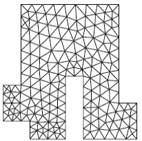
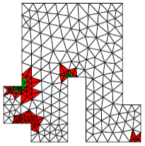
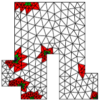
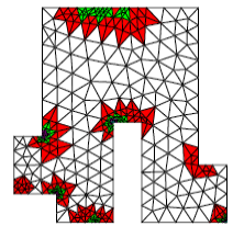
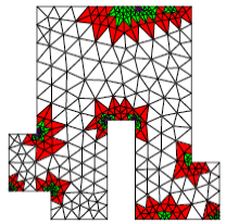
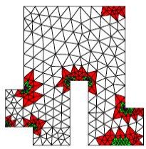
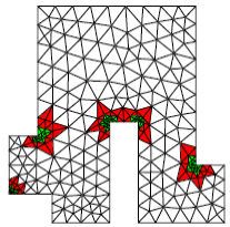
Example 6.5-2: Using the “ERTH_ELEM” option combined with HOMARD