2. Modal synthesis

Dynamic substructuring consists in determining the behavior of a structure based on the vibratory characteristics of each of its components ([bib3] and [bib4]). The methods implemented in Code_Aster simultaneously use the classical techniques of modal recombination and dynamic substructuring.

These methods, although different from that of finite elements, adopt a substantially comparable approach but nevertheless introduce an additional approximation. They reveal three essential steps:

Step 1: numerical study of each component by determining their vibratory characteristics. The work consists in identifying natural modes and static deformations using classical vibratory mechanics techniques. If you think of each substructure as a superelement, this step is similar to elementary calculation.

Step 2: connecting the substructures. The vibratory characteristics determined previously are used for each component, and their connection is taken into account. This work constitutes the sub-structuring stage itself. It is similar to an assembly.

Step 3: the resolution and an escalation phase make it possible to obtain the solution sought in the physical frame of reference of the overall structure.

2.1. Transformation of RITZ

The transformation of RITZ is the subject of the reference documentation [R5.06.01]. Here we recall its principle. For the problem of numerical determination of the real eigenmodes of the undamped system associated with the structure, which we will designate by eigenmodes, we come back to solving the following minimization problem:

For \(\delta\) virtual trip, we’re looking for: \({\mathit{Min}}_{\delta }\frac{1}{2}{\delta }^{T}\mathrm{.}(\mathrm{K}\mathrm{-}{\omega }^{2}\mathrm{M})\mathrm{.}\delta\)

whose solution :math:`` verifies:

(2.15)\[ (K-\ omega\ mathrm {²} M)\ mathrm {.} q=0\]

The method of RITZ consists in looking for the solution of the previous minimization equation on a subspace of the solution space. Consider the matrix

containing the vectors of the base of the subspace in question, organized in columns. Restricted to this small space, the minimization equation takes the following form:

\({\mathrm{Min}}_{p=\Phi \delta }\frac{1}{2}{p}^{T}\mathrm{.}(K-{\omega }^{2}M)\mathrm{.}p\)

That is the solution sought:

(2.15)\[ q=\ Phi\ eta\]

Who verifies:

(2.15)\[ (\ stackrel {} {K} -\ omega\ mathrm {²}\ stackrel {} {M})\ eta =0\]

where \(\eta\) is the vector of generalized displacements, \(\stackrel{ˉ}{K}={\Phi }^{T}K\Phi\) and \(\stackrel{ˉ}{M}={\Phi }^{T}M\Phi\) are called generalized stiffness and mass matrices respectively.

After solving the [éq 2.1-3] system, obtaining the eigenmodes in the physical base is done using the relationship [éq 2.1-2]. The transformation of RITZ therefore makes it possible to replace the initial eigenvalue problem [éq 2.1-1] by a problem of the same nature [éq 2.1-3], but of reduced dimension. The new generalized stiffness and mass matrices remain symmetric.

However, this transformation should be used with caution. In fact, since the new base is incomplete, an approximation is made at the projection level: we speak of modal truncation. The precision of the final result then depends on the choice of the basic vectors and the relative error due to this reduction in the number of unknowns must be estimated.

2.2. Modal recombination

A classic use of the RITZ transformation is dynamic analysis by modal recombination. It is commonly used to calculate the response of a structure to low frequency excitation. Here we will limit ourselves to calculating the response to an excitation of a conservative structure. In this case, the finite element method allows us to bring us back to the following matrix differential equation:

(2.15)\[ \ mathrm {M}\ ddot {\ mathrm {q}}} +\ mathrm {K}\ mathrm {q}\ mathrm {=} {\ mathrm {f}}} _ {\ mathit {ext}}\]

If we apply the transformation of RITZ, with the first eigenmodes of the structure as an incomplete basis for projection, the relationship [eq.] becomes:

(2.15)\[ \ stackrel {} {M}\ ddot {\ eta} +\ stackrel {} {K}\ eta = {\ stackrel {} {f}}} _ {\ mathrm {ext}}\]

where \({\stackrel{ˉ}{f}}_{\mathrm{ext}}={\Phi }^{T}{f}_{\mathrm{ext}}\) is the vector of generalized forces.

Eigenmodes are orthogonal with respect to mass and stiffness matrices. The differential equation [éq 2.2-2] therefore reveals diagonal matrices: the system then consists of decoupled equations. Each of them is the equation for a spring-mass single-degree oscillator that reveals the generalized mass, stiffness, and force relating to the \(j\) mode (respectively: \({m}_{j}\), \({k}_{j}\), \({f}_{j}\)) (respectively:,,), see Figure-A.

If we consider the transformation of RITZ [eq], at the level of a degree of freedom, we have:

\({q}_{i}=\underset{j}{\Sigma }{\Phi }_{\mathrm{ij}}{\eta }_{j}\)

where:

\({q}_{i}\) is the \(i\) th coordinate of the vector \(q\),

\({\eta }_{j}\) is the \(j\) th coordinate of the vector \(\eta\),

\({\Phi }_{\mathrm{ij}}\) is the component of the \(i\) th row and the \(j\) th column of the matrix \(\Phi\).

It therefore appears that the structure response is expressed as the weighted recombination of oscillator responses to a decoupled degree of freedom. The transformation of RITZ makes it possible, in this case, to define an equivalent schema of the structure, which makes the oscillators appear to have a degree of freedom associated with the identified eigenmodes. Their stiffness and mass are the generalized rigidities (\({k}_{j}\)) and the generalized masses (\({m}_{j}\)) of the corresponding modes.

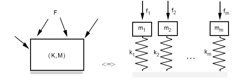
Figure -a: Principle of dynamic analysis by modal recombination.

Reserved mainly for studies that are misleadingly described as low frequencies [1] _ , modal recombination consists in using the orthogonality properties of the natural modes of a structure to simplify the study of its vibratory response. In addition to the interest of reducing the order of the numerical problem to be solved, the transformation of RITZ into a modal basis, in this case, also makes it possible to decouple the differential equations and to derive a physical interpretation of the result obtained. Depending on the excitation frequency, a more or less truncated modal base will be used. However, it is necessary to estimate the truncation error to ensure the validity of the result.

2.3. Modal synthesis

In general, modal synthesis methods consist in simultaneously using dynamic substructuring (division into substructures) and modal recombination at the level of each substructure. Often confused, by misuse of language, with dynamic substructuring, modal synthesis is only one particular case of dynamic substructuring.

Dynamic substructuring consists in considering the displacement of a substructure in the overall movement, as its response to the bonding forces that connect it to the other components and to the external forces that are applied to it.

Modal synthesis means that this movement is calculated, at the level of each substructure, by modal recombination. A projection base is therefore used that characterizes each substructure. In fact, if the overall structure is too large to be subjected to a modal calculation, the dimensions of the substructures make it possible to carry out this work. Modal synthesis requires first studying each component separately, in order to determine their projection base.

In the rest of this chapter, we present the types of modes and static deformations used in modal synthesis methods using the following simple example:

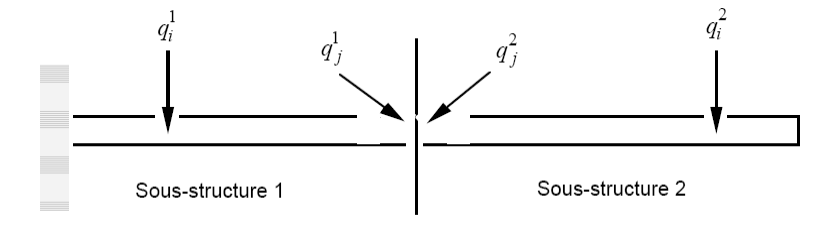
Figure -a: Principle of dynamic substructuring.

The vector of the degrees of freedom of the substructure is characterized by an exponent that defines the number of the substructure, and an index that makes it possible to distinguish internal degrees of freedom (index \(i\)), from border degrees of freedom (index \(j\)).

\({q}^{k}=\left\{\begin{array}{c}{q}_{i}^{k}\\ {q}_{j}^{k}\end{array}\right\}\)

To study substructure \(k\), it is necessary to define an impedance in terms of the degrees of freedom of the connection. As part of the developments carried out in Code_Aster, it is either zero or infinite.

The basic vectors used in the methods implemented in Code_Aster are:

• normal modes,

• constrained modes,

• the attachment methods,

• interface modes,

which is defined below.

2.3.1. The normal modes

Natural modes or normal modes are advantageously used as a basis for projecting substructures for several reasons:

• they can be calculated or/and obtained experimentally,

• they offer interesting orthogonality properties in relation to the mass and stiffness matrices of the substructure,

• they are associated with natural frequencies of the structure.

They can be of two types depending on the condition given to the connection interfaces, cf. Figures-b and -c:

• specific modes with blocked interfaces,

• specific modes with free interfaces.

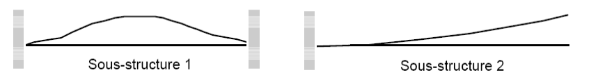
Figure -b: Modes specific to blocked interfaces.

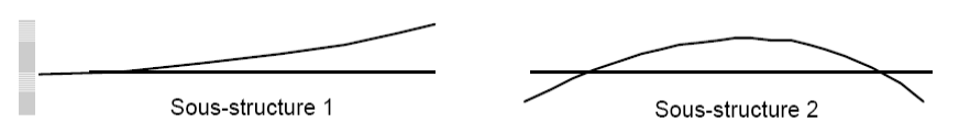
Figure -c: Modes specific to free interfaces.

Note that in the case of a free substructure, the existing rigid body modes (or set modes) are part of the transformation base.

2.3.2. Static deformations

An interface mode is defined for each degree of freedom of connection of each substructure. Depending on the case, they may be constrained modes or attachment modes.

Constrained modes are static deformations that are combined with normal modes with blocked interfaces to correct the effects due to their boundary conditions. A constrained mode is defined by the static deformation obtained by imposing a unit displacement on one degree of freedom of connection, the other degrees of freedom of connection being blocked.

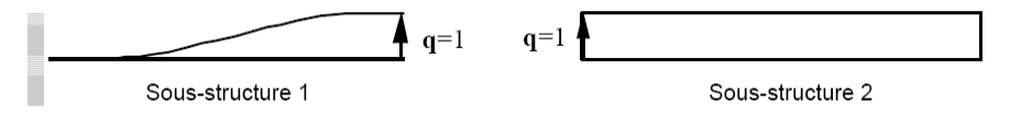
Figure -d: Constrained modes.

Attachment modes are static deformations that are combined with normal modes with free interfaces to reduce the effect of modal truncation. A mode of attachment is defined by the static deformation obtained by imposing a unitary force on one degree of freedom of connection, the other degrees of freedom of connection being free.

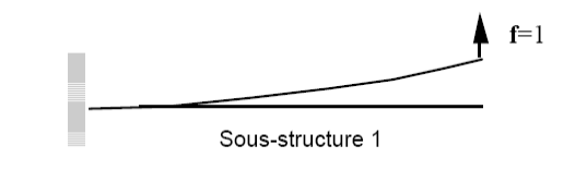
Figure -e: Attachment modes.

In the case of a substructure with rigid body modes (here, substructure2), its stiffness matrix is no longer invertible and it is not possible to calculate its attachment modes. It is then necessary to block certain degrees of freedom in order to make the structure isostatic, or even hyperstatic.

2.3.3. Harmonic deformations

A third projection base has been introduced as part of developments concerning the calculation of harmonic response by classical dynamic substructuring. This is the Craig-Bampton harmonic base.

The basis of harmonic Craig-Bampton consists of modes specific to blocked interfaces and harmonic constrained modes [bib8]. These are combined with normal modes with locked interfaces to correct the effects due to their boundary conditions. A harmonic constrained mode is defined by the response of the undamped substructure to a harmonic displacement, of a given unit amplitude and frequency, imposed on one degree of freedom of connection, the other degrees of freedom of connection being blocked.

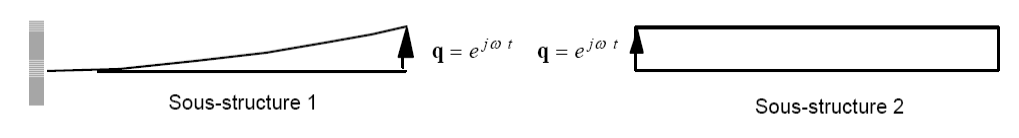
Figure -f: Harmonic constrained modes.

This modal base is more particularly suitable for fluid-structure interaction problems, for which static loads are not applicable in Code_Aster (not taking into account the added mass effect). It can be used for any type of calculation (modal, harmonic and transitory).

2.3.4. Reduced interface deformations or « coupling modes »

An interface mode is defined for all the degrees of freedom of connection of each substructure.

Interface modes are dynamic deformations that are combined with normal modes with blocked or free interfaces to correct the effects due to their boundary conditions.

Concretely, the calculation of constrained modes consists in condensing the behavior of the structure on the degrees of freedom of the interface and thus constructing an interface operator (Schur complement) that expresses the behavior of the structure reduced to the interface. By spectral analysis, it is then possible to represent the deformations of the interface by linear combination of the natural modes of this interface operator.

Figure -g: Interface mode.

2.4. Connection conditions between substructures

2.4.1. Introduction

Consider the problem of two rigidly linked substructures \({S}^{1}\) and \({S}^{2}\) that are not subject to external forces. For the movement of the complete structure to be continuous, it is necessary to impose the equality of the movements of the two components at the interface and the law of action-reaction:

(2.15)\[ \ mathrm {\ forall} M\ mathrm {\ in} {S} {S} {S} ^ {1}\ mathrm {\ cap} {S} ^ {q}} {{i}} _ {i} ^ {k} u} ^ {u} u} ^ {u} u} ^ {1} (M)\ mathrm {=} {{\ mathrm {q}}} _ {i} ^ {k} u} ^ {2} (M)\ text {and} {\ mathrm {f}}} _ {L} ^ {1} (M)\ mathrm {=}\ mathrm {-} {\ mathrm {f}}} _ {L} ^ {2} (M)\]

where:

\({u}^{1}(M)\) represents the displacement field of the substructure \({S}^{1}\),

\({u}^{2}(M)\) represents the displacement field of the substructure \({S}^{2}\),

\({f}_{L}^{1}(M)\) represents the field of the bond forces applied to the substructure \({S}^{1}\),

\({f}_{L}^{2}(M)\) represents the field of bond forces applied to substructure \({S}^{2}\).

Depending on the nature of the meshes at the interface, the previous problem may be discretized differently.

2.4.2. Case of compatible interface mesh

In this part, we limit ourselves to the case of compatible meshes. This means that they check for the following properties:

• the restriction of the meshing of each of the substructures \({S}^{1}\) and \({S}^{2}\) at the interface rely strictly on the same nodes at their intersection,

• the finite elements associated with these link cells are of the same nature (linear, quadratic) on both sides of the border.

Therefore, the condition [eq] is strictly equivalent to the formulation below:

(2.15)\[ {q} _ {{S} ^ {1}\ cap {S} ^ {1}} ^ {2}}} ^ {2}}} ^ {1}\ cap {S} ^ {2}} ^ {1}} ^ {1}\ text {and} {1}\ text {S}} ^ {1}} ^ {1}} ^ {1}}\ cap {S} ^ {2}}} ^ {1}} ^ {1}\ text {S}} {1}} ^ {1}\ text {S} {1}} ^ {1}\ text {S}} {1}} ^ {1}\ text {and} {1}\ text {and} {f} _ {f} _ {{L}} ^ {1}} _ {{L} _ {{S} ^ {1}\ cap {S} ^ {2}}} ^ {2}} ^ {2}}\]

where:

\({q}_{{S}^{1}\cap {S}^{2}}^{k}\)	is the vector of the degrees of freedom at the \({S}^{1}\cap {S}^{2}\) interface nodes of the substructure \(k\),
\({f}_{{S}^{1}\cap {S}^{2}}^{k}\)	is the vector of the binding forces at the \({S}^{1}\cap {S}^{2}\) interface nodes of the \(k\) substructure.

In fact, the meshes of the two substructures

and

coinciding on the interface, the form functions associated with the finite elements are the same at the interface. It is therefore sufficient to impose equality on the nodes of the link interfaces of each substructure to impose equality on the entire link domain.

Let’s introduce the \({B}_{{S}^{1}\cap {S}^{2}}^{k}\) interface degrees of freedom extraction matrices:

(2.15)\[ {q} _ {{S} ^ {1}\ cap {S} ^ {2}} ^ {2}} ^ {k} = {B} _ {{S} ^ {1}\ cap {S} ^ {2}}} ^ {2}}} ^ {2}}} ^ {2}} ^ {2}} ^ {k}\]

Using the projection equation [eq.], the displacement continuity condition [eq] and the above formulation applied to the two substructures, we obtain:

\({B}_{{S}^{1}\cap {S}^{2}}^{1}{\Phi }^{1}{\eta }^{1}={B}_{{S}^{1}\cap {S}^{2}}^{k}{\Phi }^{1}{\eta }^{1}\)

Either:

(2.15)\[ {L} _ {{S} ^ {1}\ cap {S} ^ {2}}} ^ {2}} ^ {2}} ^ {1} = {L} _ {{S} ^ {1}\ cap {S} ^ {2}} ^ {2}}} ^ {2}}} ^ {2}} ^ {2}}\ text {with} {L} _ {{S} ^ {1}\ cap {S} ^ {1}\ cap {S} ^ {1}\ cap {S} ^ {1}\ cap {S} ^ {1}\ cap {S} ^ {1}\ cap {S} ^ {2}} {2}}} ^ {k} = {B} _ {{S} ^ {1}\ cap {S} ^ {2}} ^ {k} {\ phi} {\ phi} ^ {k}\]

where:

\({L}_{{S}^{1}\cap {S}^{2}}^{1}\) is the link matrix of \({S}^{1}\) associated with the interface \({S}^{1}\cap {S}^{2}\), it expresses the continuity of movement between the two substructures based on the generalized displacements at the interface,

\({L}_{{S}^{1}\cap {S}^{2}}^{2}\) is the \({S}^{2}\) link matrix associated with the \({S}^{1}\cap {S}^{2}\) interface.

In the case of the problem with the eigenvalues of the global structure, provided with its boundary conditions, we can write:

(2.15)\[\begin{split} \ begin {array} {c} (\ stackrel {} {K} -\ omega\ mathrm {²}\ stackrel {} {M})\ eta + {L} ^ {T} ^ {T}\ lambda}\ lambda =0\\ L\ eta =0\ end {array}\end{split}\]

The generalized mass and stiffness matrices, the vector of the generalized degrees of freedom, and the link matrix that appear here, are defined on the overall structure. They take a form specific to each method (Craig-Bampton, MacNeal,…) which will be explained later. The Lagrange multipliers vector \(\lambda\) is interpreted by the link actions to which the interfaces are subjected.

It is therefore a classic problem of finding eigenvalues, to which a linear constraint equation is associated. In Code_Aster, this type of problem is solved by double dualization of boundary conditions [bib6].

Thus, it can be shown that this system is also a solution to the problem of minimizing the following functional, called action integral:

\(f={\int }_{a}^{b}F(\eta ,\dot{\eta },{\lambda }_{1}{\lambda }_{2})\cdot \mathrm{dt}\)

where \(\mathrm{F}(\eta ,\dot{\eta },{\lambda }_{1}{\lambda }_{2})\mathrm{=}\frac{1}{2}{\eta }^{T}\stackrel{ˉ}{\mathrm{K}}\eta +\frac{1}{2}\dot{\eta }\stackrel{ˉ}{\mathrm{M}}\dot{\eta }+{({\lambda }_{1}+{\lambda }_{2})}^{T}\mathrm{L}\eta \mathrm{-}\frac{1}{2}{({\lambda }_{1}\mathrm{-}{\lambda }_{2})}^{2}\) is the Hamiltonian.

The variables of this functional are the generalized coordinates \(\eta\), the associated speeds and the Lagrange multipliers \({\lambda }_{1}\) and \({\lambda }_{2}\) (in a number equal to 2 times the number of link equations). The last term of the functional requires the equality of the Lagrange coefficients.

The extreme is reached for the values of variables that cancel the derivatives of \(f\), regardless of whether \(a\) and \(b\) are real:

\(-{\lambda }_{1}+L\eta +{\lambda }_{2}=0\)

\({L}^{T}({\lambda }_{1}+{\lambda }_{2})+(\stackrel{ˉ}{K}-\omega \mathrm{²}\stackrel{ˉ}{M})\eta =0\)

\({\lambda }_{1}+L\eta -{\lambda }_{2}=0\)

(2.15)\[\begin{split} \ left [\ begin {array} {ccc} -\ text {Id} & L&\ text {Id}\\ {L} ^ {T} &\ stackrel {} {K} & {L} ^ {T}\\\ text {T}\\ text {Id} & L& -\\ text {Id} & L& -\ text {Id} & L& -\ text {Id}\\ text {Id} & L& -\ text {Id}\\ end {array}\ right]\ left\ {\ begin {array} {\ array} {K} & {L} ^ {T} & {L} ^ {T}\\ T}\\ T}\\ T}\\ T}\\ T}\\ text {Id} & L& -\ _ {1}\\\ eta\\\ {\ lambda} _ {2}\ end {array}\ right\} - {\ omega} ^ {2}\ left [\ begin {array} {ccc} 0& 0& 0\\ 0\\ 0\\ 0&\ 0&\ stackrel {} {M} {M} & 0\\ 0& 0& 0\ end {array}\\ right]\ left\ {\ begin {array}\ right]\ left\ {\ begin {array} c} {\ lambda} _ {1}\\\ eta\\\ eta\\\ eta\\\ {\ lambda} _ {2}\ end {array}\ right\} =\ left\ {\ begin {array} {c} {c} 0\\ 0\\ 0\\ 0\ end {array}\ right\}\end{split}\]

The double dualization therefore leads to a real symmetric matrix problem. We demonstrate [R3.03.01] that it makes it possible to make matrix triangulation algorithms unconditionally stable.

2.4.3. Case of the incompatible interface mesh

In this part, we consider the case of incompatible meshes. This means that they do not check the following properties a prima facie:

• the restriction of the meshing of each of the substructures \({S}^{1}\) and \({S}^{2}\) at the interface rely strictly on the same nodes at their intersection,

• the finite elements associated with these link cells are of the same nature (linear, quadratic) on both sides of the border.

The method chosen to manage mesh incompatibility is a method derived from that of PPCM (« Smallest Common Mesh »). This method is used in the context of several types of problems in Code_Aster: incompatible mesh management, field projection on meshes of different natures… We therefore define a « master » interface onto which we project the nodes of the « slave » interface.

The interpolation of fields to the nodes of the slave interface (elements surrounded by \({S}_{2}\) in the figure below) is done on the element of the master interface onto which each node is projected, using the shape functions of this element.

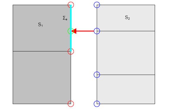
Figure -a:

We define \({\Sigma }_{e}\) as the interface restricted to one element and \({n}_{e}\) the number of ddls in the element.

By choosing the interface from substructure \({S}_{1}\) as the master interface, the relationship () is rewritten:

\({u}^{1}(M)-\sum _{j=1}^{{n}_{e}}({\int }_{{\Sigma }_{e}}{E}_{j}^{2}(M)\xi (M)\text{dM}){q}_{j}^{2}=0\)

where \(\xi (M)\) are the shape functions of the element on which the node is projected and \({E}_{j}^{2}\) is the restriction of the shape functions of the element \(j\) of the \({S}_{2}\) interface.

This method makes it possible to couple substructures with meshes of different types (linear with quadratic,…) and different densities. However, it should be noted that the rule of good use consists in choosing the mesh with the lowest density as the master.

Taking into account the conditions set out in the preceding paragraphs, the expression linking the degrees of freedoms must be rewritten. Taking the interface from substructure \({S}_{1}\) as the master interface, we have:

\({q}_{j}^{1}=\sum _{l}^{{n}_{e}}{\alpha }_{l}{q}_{l}^{2}\)

Or even:

\({q}^{1}=A{q}^{2}\)

where \(A\) is an observation matrix between the ddls of the two interfaces.

The relationships of continuity of movements are expressed, with the generalized coordinates, by the following matrix relationships:

\({L}_{j}^{1}{\eta }^{1}\mathrm{=}{\tilde{L}}_{j}^{2}{\eta }^{2}\)

\({\tilde{L}}_{j}^{k}\mathrm{=}A{B}^{k}{\Phi }^{k}\)

We can write this relationship in matrix form:

\(\left[{L}_{j}^{1}-{\tilde{L}}_{j}^{2}\right]\cdot \left[\begin{array}{c}{\eta }^{1}\\ {\eta }^{2}\end{array}\right]=0\)

The terms in the link matrices are no longer equal to zero or one. They are the result of the interpolations of the movements projected onto the elements.

Finally, using double dualization, the matrix system obtained to be solved, in the case of the modal problem on the global structure, is:

\(\Rightarrow \left[\begin{array}{ccc}-\text{Id}& \tilde{A}L& \text{Id}\\ {\tilde{A}}^{T}{L}^{T}& \stackrel{ˉ}{K}& {\tilde{A}}^{T}{L}^{T}\\ \text{Id}& \tilde{A}L& -\text{Id}\end{array}\right]\left\{\begin{array}{c}{\lambda }_{1}\\ \eta \\ {\lambda }_{2}\end{array}\right\}-{\omega }^{2}\left[\begin{array}{ccc}0& 0& 0\\ 0& \stackrel{ˉ}{M}& 0\\ 0& 0& 0\end{array}\right]\left\{\begin{array}{c}{\lambda }_{1}\\ \eta \\ {\lambda }_{2}\end{array}\right\}=\left\{\begin{array}{c}0\\ 0\\ 0\end{array}\right\}\)

Where \(\tilde{A}\) refers to the identity matrix \(\text{Id}\) if the substructure is the one whose interface is master and \(A\), the observation matrix, if it is the one whose interface is a slave.

The double dualization therefore leads to a real symmetric matrix problem even for the case of incompatible meshes.

2.4.4. Conclusion

This method therefore makes it possible to process the connection of interfaces corresponding to different types of modal bases without the cost of managing an always delicate elimination. On the other hand, it is relatively simple. The major drawback of this formulation is that it leads to final assembled systems of larger dimensions than in the case of elimination. In fact, the coupling of the matrix equations was done by introducing a number of additional degrees of freedom equal to twice the number of link equations. This increase in the dimensions of the matrices can therefore be very significant. Note that the Lagrange degrees of freedom introduced are, in this case, the forces applied at the interfaces to ensure the connection between the two substructures.

2.5. Elimination of linear constraints

The double dualization technique makes it possible to obtain uniformity in the consideration of constraints. This approach can in fact be used for both linear and non-linear constraints, on displacements or constraints. It therefore allows, with great flexibility, the carrying out of a wide variety of calculations.

However, in the context of modal analysis in general, and substructuring techniques in particular, the presence of double Lagrange multipliers may constitute a disadvantage, both linked to the increase in the size of the problem with the number of constraints, but also linked to the numerical conditioning of the system thus obtained. The increase in the size of the problem is particularly clear in the case of substructure approaches, where, for the final problem, the vast majority of the equations to be solved concern constraints. To avoid this difficulty, a technique for eliminating kinematic constraints was implemented based on a QR decomposition of the link matrices.

2.5.1. Linearly independent stress cases

The linear constraints associated with a dynamics problem can be written in the form of the linear system:

(2.15)\[ \ left [L\ right]\ cdot q=0\]

\(q\) designating all the degrees of freedom of the complete model (i.e. including all substructures, in our case). The idea of elimination is to build a core base for \(L\), and to solve the problem projected in that base. The construction of this base is done simply from the QR decomposition of \({L}^{T}\).

For a \(L\) matrix of size \(n\times N\), where \(n\) is the number of constraints, and \(N\) is the number of degrees of freedom, this decomposition is written:

(2.15)\[\begin{split} {\ left [{L} ^ {T}\ right]}} _ {N\ times n}} = {\ left [Q\ right]} _ {N\ times N}\ cdot {\ left [R\ right]}} _ {N\ times n}} _ {N\ times n}} _ {2}]} _ {N\ times n}} _ {2}]} _ {N\ right]} _ {2}]} _ {N\ right]} times (n-N)}\ right]\ cdot\ left [\ begin {array} {c} {c} {[{R} _ {1}]} _ {n\ times n}\\ {[0]}\\ {[0]} _ {(N-n)}\ {(N-n)\ times n}\ times n}\ end {array}\ right]\end{split}\]

\({Q}_{2}\) is then directly the base sought, as shown below.

2.5.2. Cases of redundant constraints

This decomposition also makes it possible to analyze what happens in the presence of redundant constraints (nodes constrained several times, « star » substructure, etc.). When the constraints are not all independent, we can write \(L\) as a linear combination of \({n}_{I}<n\) linearly independent constraints \({L}_{I}\), i.e.:

\({\left[L\right]}_{n\times N}={\left[A\right]}_{n\times {n}_{I}}\cdot {\left[{L}_{I}\right]}_{{n}_{I}\times N}\)

The decomposition of \({L}_{I}\) is written directly:

(2.15)\[\begin{split} {\ left [{L} _ {I} ^ {T}\ right]}} _ {N\ times {n} _ {I}} =\ left [{[{Q} _ {I}]} _ {N\ times {n}} _ {n} {n} {n} {n}} _ {N}} _ {I}]} _ {N\ times (N- {Q} _ {I})} _ {N\ times {n} _ {I}]} _ {N\ times {n} {n}}} _ {N\ times {n} {n}}} _ {N\ times {n} {n}}} _ {N\ times {n} {n}}} _ {N\ times {n} {n}}} _ {N\ times {n} {n}}} left [\ begin {array} {c} {[{R} _ {I}]}} _ {{n} _ {I}\ times {n} _ {I}}\\ {[0]}} _ {(N- {0]}} _ {n}} _ {n} _ {I})\ times {n} _ {i}}\ end {array}\ right]\end{split}\]

and the decomposition of \(L\) becomes:

(2.15)\[\begin{split} \ left [{L} ^ {T}\ right] =\ left [{Q} _ {I} {Q} _ {K}\ right]\ cdot\ left [\ begin {array} {c} {c} {R} _ {R} _ {R} _ {I} _ {I}\ cdot {A} _ {T}\\ 0\ end {array} {c} {c} {R} _ {R} _ {R} _ {I}\ I}\ cdot {A} ^ {T}\\ 0\ end {array} {c} {c} {R} _ {R} _ {R} _ {I}\ I\end{split}\]

\({Q}_{K}\) a \(\mathrm{Ker}(L)\) base. Indeed, for any \(q\) element in the \(L\) core, there is a vector \(y\) such as \(q=[{Q}_{K}]\cdot y\). Under these conditions, we have:

\(\begin{array}{ccc}[L]\cdot q& =& \left[\begin{array}{c}A\cdot {R}_{I}^{T}\\ 0\end{array}\right]\cdot \left[\begin{array}{c}{Q}_{I}^{T}\\ {Q}_{K}^{T}\end{array}\right]\cdot q\\ & =& \left[\begin{array}{c}A\cdot {R}_{I}^{T}\\ 0\end{array}\right]\cdot \left[\begin{array}{c}{Q}_{I}^{T}\\ {Q}_{K}^{T}\end{array}\right]\cdot \left[{Q}_{K}\right]\cdot y\\ & =& [A\cdot {R}_{I}^{T}]\cdot [{Q}_{I}^{T}]\cdot [{Q}_{K}]\cdot y\\ & =& 0\end{array}\)

since \(I(L)\) and \(\mathrm{Ker}(L)\) are orthogonal. When the constraints of \(L\) are linearly independent, we have \({Q}_{K}={Q}_{2}\) directly. If not, you must build \({Q}_{K}\) from \({Q}_{2}\) and the columns \(n-{n}_{I}\) last columns from \({Q}_{1}\).

To identify the rank \({n}_{I}\) of the matrix \(L\), we use the upper triangular matrix \({R}_{1}\), resulting from the relationship (). According to the relationship (), it should in fact take the form:

\({\left[{R}_{1}\right]}_{n\times n}=\left[\begin{array}{c}{[{R}_{I}]}_{{n}_{I}\times {n}_{I}}\cdot {[A]}_{n\times {n}_{I}}^{T}\\ {[0]}_{(n-{n}_{I})\times n}\end{array}\right]\)

Rank \({n}_{I}\) is the number of non-zero diagonal terms in \({Q}_{1}\). As a result, the vectors of \({Q}_{1}\) belonging to the core of \(L\) are therefore those corresponding to the zero diagonal terms of \(R\). In practice, the search for \({n}_{I}\) is dependent on the value set as the threshold for the numerical zero.

2.5.3. Case of a large number of constraints

The principles set out in the preceding paragraphs can be implemented numerically as they are and maintain correct performances if the matrices associated with the constraints are of limited size, i.e. a maximum of the order of a thousand constraints, involving of the order of ten thousand degrees of freedom. Otherwise, one of the methods consists in constructing this subspace iteratively.

The overall approach consists in successively modifying the rows of the matrix \(Q\), for all the constraints of \(L\). The starting matrix \(Q\) is the identity matrix. To illustrate the approach, let’s consider a particular step by choosing a set of constraints from \(L\). We note \({Q}_{k}\) the matrix taking into account the elimination of the first \(k\) constraints. The construction of \({Q}_{k+1}\) is done in the following way:

• Extract line \({L}_{k+1}\) from \(L\),

• Determine the number of non-zero elements in \({L}_{k+1}\). These non-zero elements are associated with the degrees of freedom involved in the linear relationship of the type of ().

  • If a single element of \({L}_{k+1}\) is non-zero, we cancel the \({Q}_{k+1}\) diagonal term associated with this degree of freedom.

  • If several non-zero elements are detected, using the previous \({L}_{k}\) lines, we look for what degrees of freedom are already involved in a linear relationship. The sub-matrix of \({\mathrm{Q}}_{k+1}\) is constructed to eliminate the new constraints taking into account the presence of the previous constraints.

For this last point, we note \({q}_{i}\) the degrees of freedom involved in the \({L}_{k}\) previous linear relationships, and \({q}_{l}\) the other degrees of freedom. The linear relationship subset associated with \({L}_{k+1}\) is therefore written \([{L}_{i}{L}_{l}]\left\{\begin{array}{c}{q}_{i}\\ {q}_{l}\end{array}\right\}=0\), and we are looking for the block of \({Q}_{k+1}\) that verifies \([{L}_{i}{L}_{l}]\left[\begin{array}{cc}{Q}_{ii}& {Q}_{il}\\ {Q}_{li}& {Q}_{ll}\end{array}\right]=0\). Block \({Q}_{\mathrm{ii}}\) was built beforehand, and should not be modified to avoid impacting the \({L}_{k}\) previous relationships. So we build \({Q}_{il}\), \({Q}_{li}\) and \({Q}_{ll}\) such as:

• • • \({Q}_{il}=0\),

    • \({Q}_{li}=-{({L}_{l})}^{\text{+}}{L}_{i}{Q}_{ii}\), where \({({L}_{l})}^{\text{+}}\) is the pseudo-inverse of \({Q}_{l}\), allowing to solve \({L}_{i}{Q}_{ii}+{L}_{l}{Q}_{li}\mathrm{=}0\),

    • \({Q}_{ll}\) is built by decomposing \(QR\) from \({L}_{l}={Q}_{ll}{R}_{ll}\). After decomposition, the columns of \({Q}_{ll}\) associated with the non-zero diagonal terms of \({R}_{lŀ}\) are set to zeros.

Several choices exist for the successive construction of \({L}_{k}\), and consist either in extracting a fixed number of lines from \(\mathrm{L}\) for each step, or in doing a search for disjoint constraint blocks in \(L\).

[1]

Frequency range over which the natural frequencies of the structure are distinguishable, generally the first frequencies of a structure.