2. Evolutionary Kanai-Tajimi DSP model#
Kanai-Tajimi’s DSP model [bib13], which expresses filtered white noise and models seismic acceleration in a free field, is one of the most classical. The two parameters of the original Kanai-Tajimi model are therefore the natural pulsation of the filter as well as the damping of the latter. This model has evolved since then, in particular with regard to the filtering of low-frequency content [bib2] and the introduction of the evolution of the frequency content of seismic signals (Ahmadi & Fan [bib1] )) . Low frequency filtering makes it possible to obtain accelerating signals that can be integrated without drifts in movement and speed (it is necessary to use « *baseline correction » if integration constants must be eliminated). Finally, a modulation function is applied in order to obtain the amplitude variation. This model is implemented in*Code_Aster and*available via operator GENE_ACCE_SEISME, option DSP* . *
2.1. General formulation of the model#
The model selected is summarized as follows:
The \(Y\) process is characterized by the DSP of Kanai-Tajimi (KT): this DSP models the absolute acceleration response of a mass subjected to excitation by white noise (the seismic movement at the rock). In other words, Kanai-Tajimi’s DSP describes white noise filtered by an oscillator with a natural pulsation \({\omega }_{0}\) and reduced damping \({\xi }_{0}\).
The fundamental pulse \({\omega }_{0}\) of the DSP of evolutionary KT is a function of time:
\({S}_{\mathit{KT}}(\omega ,t)=\frac{({\omega }_{0}{(t)}^{4}+4{\xi }_{0}^{2}{\omega }_{0}{(t)}^{2}{\omega }^{2})}{({({\omega }_{0}{(t)}^{2}-{\omega }^{2})}^{2}+4{\xi }_{0}^{2}{\omega }_{0}{(t)}^{2}{\omega }^{2})}{S}_{0}\) (10)
A linear evolution of the natural pulsation with respect to time is assumed during the strong phase of the earthquake:
\({\omega }_{0}(t)=\{\begin{array}{cc}{\omega }_{1}& \mathrm{si}t<{t}_{1}\\ {\omega }_{1}-\omega \text{'}(t-{t}_{m})& \mathrm{si}{t}_{1}<t<{t}_{2}\end{array}\) (11)
where \({t}_{1}\) and \({t}_{m}\) respectively designate the beginning and the middle moment of the strong phase: \({t}_{m}=0.5({t}_{1}+{t}_{2})\) (see also §1.2 for a definition of these quantities). For \(t<{t}_{1}\) the natural pulsation is assumed to be constant equal to \({\omega }_{1}={\omega }_{0}({t}_{1})\).
For \(t>{t}_{2}\), the natural pulsation is assumed to be constant equal to \({\omega }_{2}={\omega }_{1}-\omega \text{'}({t}_{2}-{t}_{1})\). The user must ensure that the natural pulsation given by this relationship remains positive over time.
Filtering KT’s DSP by a :math:`{omega }_{f}` natural pulsation filter and a reduced damping :math:`{xi }_{f}=1.0` according to Clough & Penzien (CP). This filtering makes it possible to remove very low frequency content that leads to non-zero drifts (non-zero movements and speeds at the end of the earthquake). In the*Code_Aster implementation, we take \({\omega }_{f}=0.05{\omega }_{0}\) by default, but the user can provide other values if they want. Seismologists call frequency \({\omega }_{f}\) « Corner Frequency », which is the minimum frequency below which the spectrum should tend towards 0. This leads us to DSP fixed \({S}_{\mathrm{CP}}(\omega )\):
\({S}_{\mathrm{CP}}(\omega ,t)=∣h(\omega )∣{}^{2}{S}_{\mathrm{KT}}(\omega ,t)\), where the filter is written \(h(\omega )=\frac{{\omega }^{2}}{({\omega }_{f}^{2}-{\omega }^{2}+\mathrm{2i}{\xi }_{f}{\omega }_{f}\omega )}\)
Two temporal modulation functions for amplitude \(q(t)\) are proposed: the gamma function and the Jennings & Housner function [bib4]. These functions and their settings are described in Chapter 1.
The evolution of the fundamental pulsation of the evolutionary Kanai-Tajimi model is illustrated in Figure 1a. Figure 2a shows filtered Kanai-Tajimi DSP (DSP by Clough & Penzien) for a given natural frequency. For regular DSP functions, the natural frequency of the filter is close to the fundamental frequency of DSP. In FIG. 1, we also visualize the width of the band of DSP, noted \(\delta\). The width of the band of DSP is linked to the damping of the filter as explained in §3.1.
Note:
A model very similar to the one described above is proposed in the reference (Rezaeian & Der Kiureghian, [bib9,bib10]). The difference between the two approaches is mainly in writing the problem in the time domain by Rezaeian & Der Kiureghian and not in the frequency domain through the spectral density as proposed here. However, writing in the time domain has a number of disadvantages, such as the need to evaluate the convolutional integral and to work with the Wiener process (white noise), which is not a second-order process. The formulation of the problem by filtered white noise described by its evolving DSP as proposed here is, on the other hand, very easy and numerically much more effective.
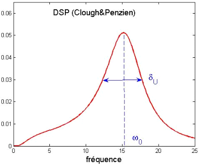
Figure 2a DSP of Kanai-Tajimi after filtering the low frequencies according to Clough & Penzien [bib2].
2.2. Setting up the modulation functions#
The parameters that characterize the shape of the modulation function are the duration of the strong phase \({T}_{\mathrm{SM}}\), the moment of the start of the strong phase \({t}_{\mathrm{ini}}\). The amplitude of the signals to be generated is determined by the Arias intensity data \({I}_{a}\) (energy), the standard deviation \({\sigma }_{X}\) over the duration of the strong phase, or the median maximum \({a}_{m}\) over the duration of the strong phase.
Data are assumed to be the averages of these parameters, in particular the duration of the mean strong phase \(\stackrel{ˉ}{T}{}_{\mathrm{SM}}\), the time of the beginning of the strong mean phase \(\stackrel{ˉ}{{t}_{\mathrm{ini}}}\) and the average Arias intensity \({\stackrel{ˉ}{I}}_{a}\).
In practice, the median maximum \({a}_{m}\) is associated with the PGA data (Peak Ground Acceleration). Thus, if PGA is given, then it is considered that this one corresponds to the median of the maxima \({a}_{m}=\mathrm{Médiane}({\mathrm{max}}_{t\in T}(∣X(t)∣))\) of the process trajectories (during the strong phase \(T{}_{\mathrm{SM}}\)). This allows us to determine the standard deviation \({\sigma }_{X}\) corresponding to this maximum using the peak factor \({\eta }_{{T}_{\mathrm{SM}}}\):
\({a}_{m}\approx {\eta }_{{T}_{\mathrm{SM}}}{\sigma }_{X}\) (8)
The peak factor is given by the formula
\({\eta }_{{T}_{\mathrm{SM}},p}^{2}=2\mathrm{ln}({\mathrm{2N}}_{\eta }[1-\mathrm{exp}(-{\delta }^{1.2}\sqrt{\pi \mathrm{ln}({\mathrm{2N}}_{\eta })})])\) (9)
where \({N}_{\eta }=\mathrm{1,4427}{T}_{\mathrm{SM}}{\nu }_{0}^{+}\). The variables \({\nu }_{0}^{+}\) (center frequency) and \(\delta\) (width of the band) are calculated from the moments of the DSP according to the expression (17) in §3.1.
The average Arias intensity \({\stackrel{ˉ}{I}}_{a}\) of a \(Y(t)\in ℝ\) process modulated by a function \(q(t)\), described by equation (1), is expressed as:
\(\stackrel{ˉ}{{I}_{a}}=E(\frac{\pi }{2g}{\int }_{0}^{\infty }{X}^{2}(t)\mathrm{dt})=\frac{\pi }{2g}{\int }_{0}^{\infty }{q}^{2}(t)E({Y}^{2}(t))\mathrm{dt}\) (4)
knowing that \(X(t)=q(t)Y(t)\). The operator \(E\) in the expression above refers to the mathematical expectation and \(g\mathrm{=}\mathrm{9.81m}\mathrm{/}{s}^{2}\). If we standardize the \(Y(t)\) process so that \({\sigma }_{Y}(t)=1\), we can write:
\(\stackrel{ˉ}{{I}_{a}}=\frac{\pi }{2g}{\int }_{0}^{\infty }{q}^{2}(t)\mathrm{dt}\) (5)
In practice, the integration takes place up to the end moment \(T\) of the seismic signals. The duration of the strong mean phase \(\stackrel{ˉ}{T}{}_{\mathrm{SM}}\) is defined from the Arias intensity, which expresses the energy contained in the seismic signal. Thus, \(\stackrel{ˉ}{T}{}_{\mathrm{SM}}\) is defined as the length of time between the time moments \({t}_{0.05}\) and \({t}_{0.95}\) where respectively 5% and 95% of the Arias intensity is achieved. The moment \({t}_{0.05}\) therefore refers to the start of the strong medium phase, \(\stackrel{ˉ}{t}{}_{\mathrm{ini}}\), such as:
\(\stackrel{ˉ}{t}{}_{\mathrm{ini}}:\frac{\pi }{2g\stackrel{ˉ}{{I}_{a}}}{\int }_{0}^{{t}_{\mathrm{ini}}}{q}^{2}(t)\mathrm{dt}=0.05\) (6)
and \(\stackrel{ˉ}{t}{}_{\mathrm{ini}}+\stackrel{ˉ}{T}{}_{\mathrm{SM}}\) the end of the strong phase:
\(\stackrel{ˉ}{t}{}_{\mathrm{ini}}+\stackrel{ˉ}{T}{}_{\mathrm{SM}}:\frac{\pi }{2g\stackrel{ˉ}{{I}_{a}}}{\int }_{0}^{\stackrel{ˉ}{t}{}_{\mathrm{ini}}+\stackrel{ˉ}{T}{}_{\mathrm{SM}}}{q}^{2}(t)\mathrm{dt}=0.95\) (7)
Given the duration of the strong phase, the average Arias intensity \({\stackrel{ˉ}{I}}_{a}\) makes it possible to determine the standard deviation of the \(X\) process.
**Note:**The parameters of the modulation functions are determined from the mean strong phase and the mean Arias intensity, as described above. The strong phases, maxima (PGA) and Arias intensities of the seismic signals generated with this modeling will therefore show a certain variability around the averages.
2.3. Uncertainties and natural variability of signals#
The parameters of the Kanai-Tajimi model are:
The average duration of the strong phase \(\stackrel{ˉ}{T}{}_{\mathrm{SM}}\) and the moment of start of the strong medium phase \(\stackrel{ˉ}{t}{}_{\mathrm{ini}}\) (modulation function),
The natural pulsation \({\omega }_{1}\) and the slope \(\omega \text{'}\) of the of Kanai-Tajimi’s DSP (or \({\omega }_{0}\) if we consider a constant value),
Reduced amortization \({\xi }_{0}\) of the DSP of Kanai-Tajimi,
The average Arias intensity \({\stackrel{ˉ}{I}}_{a}\) (average energy contained in the seismic signal), the PGA (median maximum \({a}_{m}\)) or the standard deviation \({\sigma }_{X}\).
In order to better represent the natural variability of seismic signals and to take into account the uncertainty in the parameters of the model, they can be modelled by random variables. Each simulated seismic signal then corresponds to a particular drawing of the parameters of the model. The Latin Hypercube drawing method is an effective method that makes it possible to clearly scan the field of parameter definition for a small number of draws.
The average values as well as the distributions of these parameters can be estimated from natural seismic signals corresponding to the scenario sought. Some of them are also available in the literature. A very comprehensive treatment can be found in reference [bib9]. Means, minimum and maximum values and distributions of the parameters, identified from accelerograms recorded on medium to hard ground and \(D>\mathrm{10km}\) (from the NGA [bib14] earthquake database), are presented in the appendix of this document. These results are taken from the report by Rezaeian & Der Kiureghian [bib9].