2. Model of metallurgical behavior under cooling#
2.1. Introduction#
Based on the dilatometry test [r4.04.01-Dilato], the only knowledge, At a given moment, the temperature of a steel undergoing structural transformations does not does not allow to know its state of deformation. On the other hand, the behavior of such steel seems be able to be described in the framework of models of behavior with internal variables [biB6] _. In fact, if we introduce:
- \(Z=\left\{{Z}_{i}; \; i=1,p \right\}\) the \(p\) -tuple of the proportions of
possible metallurgical components present at a point \(M\) and at an instant \(t\) given (here, \({Z}_{1}+{Z}_{2}+{Z}_{3}+{Z}_{4}\) will be the proportions of ferrite, pearlite, bainite and martensite and the proportion of austenite in \(M\) will be equal to \({Z}_{\gamma} = 1-\left ({Z}_{1}+{Z}_{2}+{Z}_{3}+{Z}_{4}\right )\));
- The thermal deformations of austenite \({\varepsilon }_{\gamma }^{\mathrm{th}}\left (T\right )={\alpha }_{\gamma }\left (T-{T}^{\gamma }\right )\)
and ferritic, pearlitic, bainitic and martensitic phases \({\varepsilon }_{\alpha }^{\mathrm{th}}\left (T\right )={\alpha }_{\alpha }\left (T-{T}^{\gamma }\right )+\Delta {\varepsilon }_{\alpha\gamma }\left ({T}^{\gamma }\right )\) by noting:
The average thermal expansion coefficient of austenite \({\alpha }_{\gamma }\);
- The reference temperature \({T}^{\gamma }\) at which we consider
\({\varepsilon }_{\gamma }^{\mathrm{th}}\) null;
- The average thermal expansion coefficient \({\alpha }_{\alpha }\) assumed
the same for ferrite, pearlite, bainite, and martensite;
- Deformation \(\Delta {\varepsilon }_{\alpha \gamma }^{\gamma }\), at the
temperature \({T}^{\gamma }\), ferritic, pearlitic, bainitic phases and martensitic with respect to austeniteleft (taking the latter as the reference phaseright);
If we consider, in addition, that the deformation of a multiphase mixture can be obtained from deformations of each phase by a linear mixing law, we can then describe the evolution of the state of deformation during a dilatometric test by:
: label: EQ-DeFotherMulti1
{varepsilon} ^ {mathrm {th}}left (Z, Tright) =left (1-sum _ {i=1} ^ {i=4} {Z} _ {i}right) {i}right) {varepsilon}) {varepsilon}} _ {gamma} ^ {mathrm {th}}left (Tright) +left (sum _ {i=1} ^ {i=4} {Z} {Z} _ {i}right) {varepsilon} _ {alpha} ^ {mathrm {th}}}left (Tright)
either
: label: EQ-DeFotherMulti2
{varepsilon} ^ {mathrm {th}}}left (Z, Tright) =left (1-sum _ {i=1} ^ {i=4} {Z} _ {i}right)left [{i}right)right)right)right)left)left [{alpha} _ {alpha} _ {alpha} _ {alpha} _ {alpha} _ {alpha} _ {alpha} _ {alpha} _ {alpha} _ {alpha} _ {alpha} _ {alpha} _ {alpha} _ {alpha} _ {alpha} _ {alpha} _ {alpha} _ {alpha} _ {alpha} _ {alpha} _ {alpha} _ {alpha} {i=1} ^ {i=4} {Z} _ {i}right)left [{alpha} _ {alpha}left (T- {T} ^ {gamma}right) +Delta {gamma}right) +Delta {gamma}right) +Delta {gamma}right) +Delta {varepsilon} _ {alpha} _ {alpha} _ {gamma}right]
The problem then lies in the determination of \(Z\) or, more precisely and within the framework simple materials with internal variables, in the determination of the evolution function \(f\) such as: \(\dot{Z}=f\left (T,Z,\cdots\right )\).
To account for an effect of the cooling rate on the evolution of transformations structural, we propose, in the context of simple materials with internal variables, a modeling of the metallurgical behavior of steels under cooling which includes, a principle, \(\dot{T}\) among its state variables.

2.2. Assumptions#
Hypothesis H1: A steel capable of undergoing structural transformations is a simple material with internal variables among which we can choose the quadruplet \(Z\) characterizing the metallurgical structure at a given point and at a given time. We therefore model structural transformations at a scale where the material point can be multiphase. This modeling scale, which may appear metallurgically crude, is consistent with the concept of material point used in the mechanics of continuous media and of which the dilatometry test piece, which is assumed to be homogeneous, is representative. |
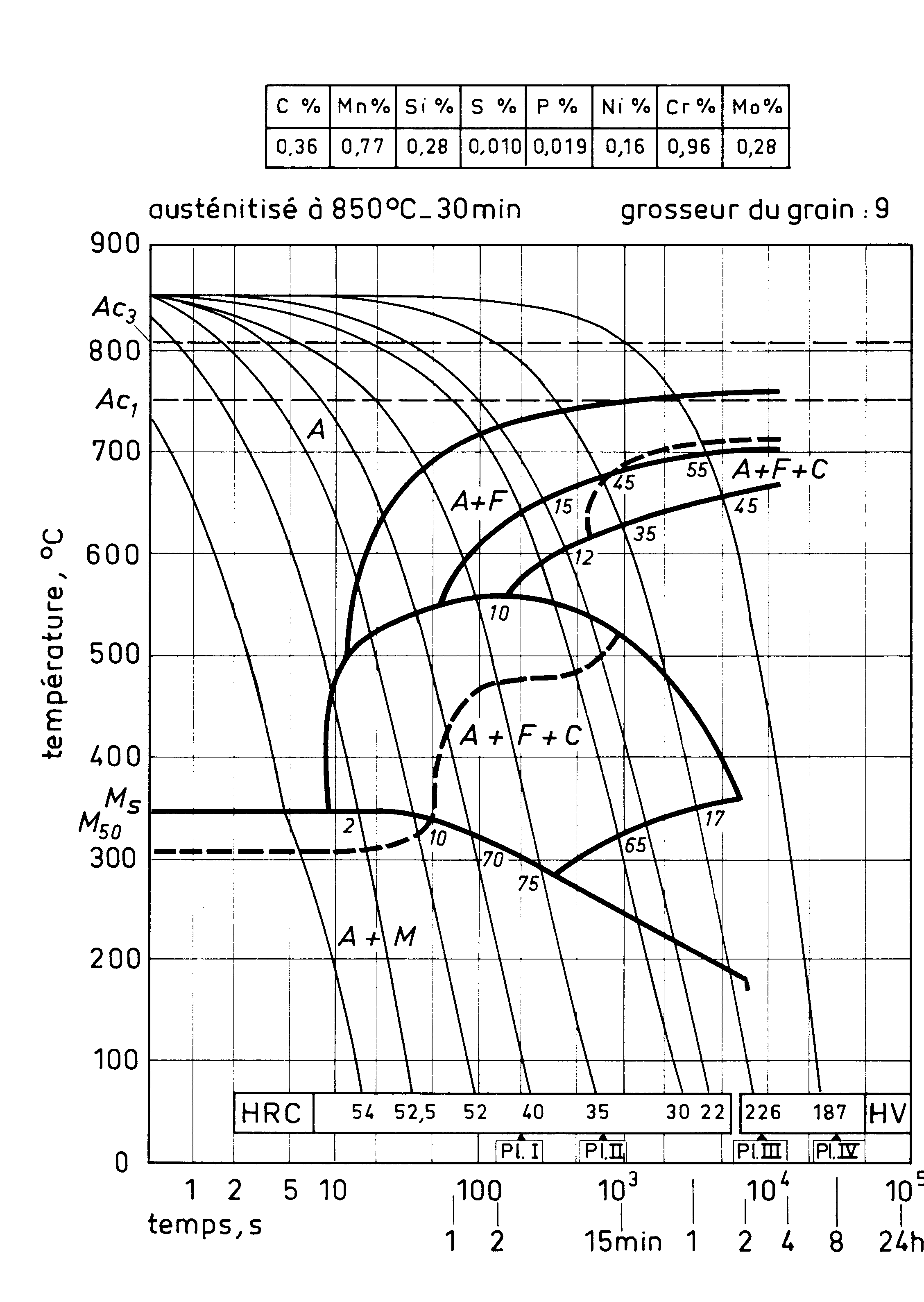
Hypothesis H2: The completed diagrams TRC of the martensitic transformation kinetics of Koïstinen-Marbürger [bib7] _ completely characterize metallurgical behavior of austenitized steel during continuous cooling. This hypothesis results directly from metallurgical practice and specifies the first of objectives to be set for the model: to be compatible with all the relative experimental data to the metallurgical behavior that accompanies the cooling of austenitized steels. Moreover, this hypothesis also creates a « natural » choice and restrictions on variables to be introduced into the model.
Hypothesis H3: Ferritic, pearlitic, and (especially) bainitic transformations are impossible below the starting temperature of the martensitic transformation:math: {M} _ {s} . | This hypothesis, in accordance with the representation of diagrams TRC, makes it possible to decouple the transformations by diffusion of the martensitic transformation. |
2.3. Choice of state variables#
Pilot state variables
In thermo-mechanics of continuous media, the pilot state variables are generally the temperature and the state of stresses or deformations. However, due to the H2hypothesis, temperature is the only pilot variable selected. In fact, the influence of the stress state on structural transformations does not appear in diagrams TRC. In addition, there is no model (except for a Le Châtelier effect) theoretical even if experimental data relating to this influence under isothermal conditions were obtained for certain steels [bib8] _.
Internal state variables
The first internal variable to be introduced is the quadruplet \(Z\) characterizing the metallurgical structure and whose knowledge is sufficient, a prima facie, to describe from a point of view mechanical a dilatometric test.
Besides the temperature \(T\), its derivative \(\dot{T}\) and the stress state \(\sigma\), The austenitic grain size \(d\) and the carbon content \(C\) of austenite se transformers also influence the metallurgical behavior of steels when cooled. However, still due to the H2 hypothesis, we choose not to introduce \(C\) as internal variable. Indeed, carbon diffusion does not appear explicitly on diagrams TRC, although it is implicitly taken into account, at least partially, in the very concept of metallurgical component.
Furthermore, Giusti [bib10] _ showed that if taking \(C\) into account was theoretically possible, it led to evolution equations coupled between \(C\) and \(Z\) whose experimental identification « seems very difficult, if not impossible » [bib9] _.
However, an effect of carbon content on the decomposition of austenite upon cooling appears indirectly on diagrams TRC. It is the phenomenon of stabilization of austenite which results in a decrease in the martensitic transformation temperature \({M}_{s}\) [:ref:r4.04.01-ExempleTRC`].
In contrast to the carbon content, the austenitic grain size \(d\) appears on diagrams TRC which relate to austenitization conditions to which a value of \(d\). So we choose to introduce \(d\) as an internal variable. However, the austenitic grain size, which results from the thermal history experienced during heating no longer evolves when cooled and \(d\) only intervenes as a parameter in the cooling behavior model.
Moreover, the martensitic transformation temperature \({M}_{s}\), which depends on the thermo-metallurgical history undergone, intervenes in the Koïstinen-Marbürger law adopted in the H2 hypothesis to describe the martensitic transformation. We therefore choose to introduce \({M}_{s}\) as an internal variable.
The memory nature of the internal variables introduced here in addition to \(Z\) appears clearly: \(d\) characterizes the thermal history suffered during the transition to the austenitic phase and \({M}_{s}\) relates the decomposition of austenite to the conditions of its transformation into martensite.
The CALC_META operator’s ACIER relationship has nine internal variables:
Variable |
Quantity |
Description |
|---|---|---|
|
20 |
50 |
\(\mathrm{V1}\) |
\({Z_1}\) |
ferrite proportion |
\(\mathrm{V2}\) |
\({Z_2}\) |
proportion of pearlite |
\(\mathrm{V3}\) |
\({Z_3}\) |
proportion of bainite |
\(\mathrm{V4}\) |
\({Z_4}\) |
proportion of martensite |
\(\mathrm{V5}\) |
\({Z_\gamma}\) |
proportion of austenite (hot phase) |
\(\mathrm{V6}\) |
\({Z_c}\) |
proportion of cold phases |
\(\mathrm{V7}\) |
\(d\) |
austenitic grain size |
\(\mathrm{V8}\) |
\(T_g\) |
temperature at Gauss points |
\(\mathrm{V9}\) |
\({M}_{s}\) |
martensitic transformation temperature |
It is also necessary to model all the phenomena involved during a welding operation to introduce other internal variables such as the tensors of anelastic deformations that can correspond to plastic deformations, of plasticity transformation or viscosity. But, in accordance with the H2 hypothesis, it is considered that these variables do not intervene in the evolution functions of \(Z\) and \({M}_{s}\).
Finally, the following hypotheses make it possible to simplify and further specify the general form of the model:
Hypothesis H4: The spatial temperature gradient \(\nabla T\) is only involved in the relationship of behavior expressing the heat current vector \(q\); its first time derivative \(\dot{\mathrm{\nabla }T}\) is not a state variable and the behavior relationship Expressing the heat current vector is Fourier’s law \(q\mathrm{=}{-}\lambda \left (T,Z,d\right )\mathrm{\nabla }T\).
Hypothesis H5: A TRC diagram identifies an empirical relationship between \({M}_{s}\), \(d\) and \(\sum _{i=1}^{i=3}{Z}_{i}\)
: label: EQ-RelaOther Vari
{M} _ {s}left ({Z} _ {1}, {1}, {Z} _ {1}, {Z} _ {3}; dright) = {{M} _ {s}} _ {0}left (dright) +Aleft (dright) +Aleft (dright) +Aleft (dright) +Aleft (dright) +Aleft (dright) {left (dright) {left [left (dright)] {left [left (dright)] {left [left] (dright) {left [sum _ {i=1} ^ {i=3} {Z} _ {i} - {Z} ^ {s} _ {gamma}left (dright)right]} ^ {+}
Hypothesis H5 means that the temperature at which the start of martensitic transformation is constant (for a given grain size) and equal to \({{M}_{s}}_{0}\) as long as the proportion of transformed austenite is less than a threshold \({Z}^{s}_{\gamma}\) and that its variation is a linear function of the quantity of austenite transformed (with the linearity coefficient \(A\left (d\right )\)). This hypothesis seems to be relatively well verified experimentally. It allows you to exclude \({M}_{s}\) of all behavioral relationships other than the one expressing \(z\) and \({Z}_{4}\).
With \(z=\left\{{Z}_{1}, {Z}_{2}, {Z}_{3} \right\}\) that will be easy to distinguish of \(Z=\left\{{Z}_{i}; \; i=1, p\right\}\) defined previously.
Finally, taking into account the H2 and H3 hypotheses, the relationships defining the model are written: so for cold phases (excluding martensite)
: label: EQ-EquaDiff Cold Phases
dot {z}left (tright) =fleft (T,dot {T}, z, {M} _ {s}; dright) =fleft (T,dot {T}, z; z; dright) {right) {frac {right) {frac {left [T- {M}} _ {s}}}} ^ {+}}
with \(z=\left\{{Z}_{1},{Z}_{2},{Z}_{3}\right\}\)
For martensite, the phase is written (Koïstinen-Marbürger equation, see [bib7] _)
: label: EQ-Koistinenmarburger
{Z} _ {4}left (T, z, {M} _ {M} _ {s}; dright) =left [1-sum _ {i=1} ^ {i=3} {Z} {Z} _ {i}right]left]left{i}right]left{i}right]left{i}right]leftleft{i}right]leftleft{i}right]leftleft{i}right]leftleft{i}right]leftleft{i}right]leftleft{i}right]leftleft{i}right]leftleft{1-expleft (1-expleftright]rightrbrace ^ {+}right)right}
and the martensitic transformation temperature
: label: EQ-Transfomartensite
{M} _ {s}left (tright) = {{M} _ {s}}} _ {0}left (dright) + {A}left (dright) {left [sum _ {i=1} {i=1}} ^ {i=1} ^ {1}} ^ {right)right]} ^ {+}
where: \(\beta\) is a characteristic of the material (of dimension \(°{C}^{-1}\)), possibly a function of \(d\) and \({[X]}^{\text{+}}\) denotes the positive part of \(X\).
Finally, as it seems difficult to propose a simple form of dependence of the model on
For these variables, we chose not to impose any particular form on the evolution functions
\({f}_{i}\) [bib2] _. The process for calculating the rates of change of variables
metallurgical then uses interpolation techniques and is based on the fact that all
Experimentally known thermometallurgical history (dilatometric test for example) is a
particular solution of the differential evolution equation eq-equaDiffPhasesFroides.