4. Elastic absorbent elements in code_aster#
This part presents most of the general constraints for implementing absorbent elastic border elements with the paraxial approximation of order 0 in code_aster. We recall the paraxial impedance relationship of order 0 as established by Modaressi for a linear elastic domain:
\(\mathrm{t}\left(\mathrm{u}\right)=\mathrm{\rho }\left({c}_{p}\frac{\partial {\mathrm{u}}_{\phantom{\mathrm{.}}\perp \phantom{\mathrm{.}}}}{\partial t}+{c}_{s}\frac{\partial {\mathrm{u}}_{\text{//}}}{\partial t}\right)\)
\({\mathrm{u}}_{\mathrm{T}}\) becomes \({\mathrm{u}}_{3}\) and \({\mathrm{u}}_{\text{//}}\) becomes \({\mathrm{u}}^{\text{/}}\)
4.1. Adaptation of seismic loading to paraxial elements#
In the first part, the principle of taking into account the incident field using paraxial elements was presented. Here it is appropriate to present the methods for modeling seismic loading in code_aster in order to be able to adapt the data to the requirements of paraxial elements.
The fundamental dynamic equation associated with any 2D or 3D model discretized in finite elements of a continuous medium or structure and in the absence of external loading is written in the absolute coordinate system:
\(\mathrm{M}{\ddot{\mathrm{X}}}_{\mathrm{a}}+\mathrm{C}{\dot{\mathrm{X}}}_{\mathrm{a}}+{\text{KX}}_{\mathrm{a}}=0\)
The movement of the structures is broken down into a driving movement \({\mathrm{X}}_{\mathrm{e}}\) and a relative movement \({\mathrm{X}}_{\mathrm{r}}\).
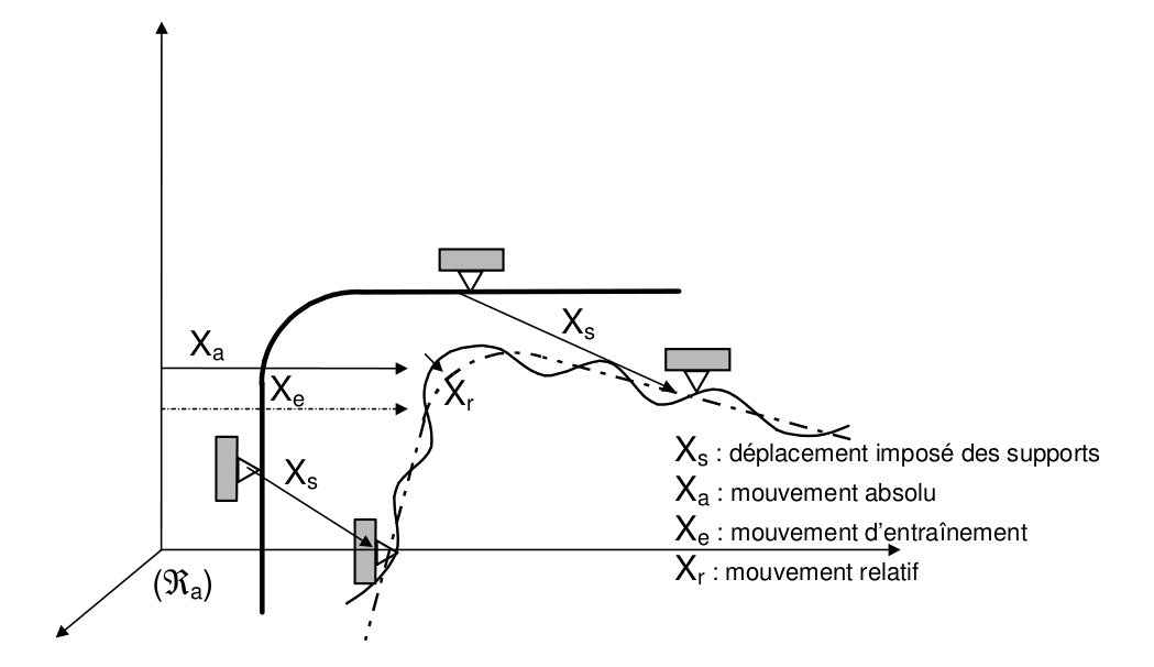
Figure 4.1-a: Breakdown of the movement of structures
So, \({\mathrm{X}}_{\mathrm{a}}={\mathrm{X}}_{\mathrm{r}}+{\mathrm{X}}_{\mathrm{e}}\)
\({\mathrm{X}}_{\mathrm{a}}\) is the vector of movements in the absolute coordinate system,
\({\mathrm{X}}_{\mathrm{r}}\) is the vector of relative displacements, that is to say the vector of the displacements of the structure in relation to the deformation that it would have under the static action of the displacements imposed on the supports \({\mathrm{X}}_{\mathrm{S}}\). So \({\mathrm{X}}_{\mathrm{r}}\) sucks at anchor points,
\({\mathrm{X}}_{\mathrm{e}}\) is the vector of the training movements of the structure produced statically by the imposed displacement of the supports \({\mathrm{X}}_{\mathrm{S}}\): \({\mathrm{X}}_{\mathrm{e}}=\mathrm{\Psi }{\mathrm{X}}_{\mathrm{s}}\),
\(\mathrm{\Psi }\) is the static mode matrix. Static modes represent the response of the structure to a unitary displacement imposed at each degree of freedom of connection (the others being blocked), in the absence of external forces. So \(\mathrm{K}\mathrm{\Psi }=0\), that is, \({\text{KX}}_{e}=0\).
In the case of mono-support (all supports undergo the same imposed movement), \(\mathrm{\Psi }\) is a rigid body mode.
Assumption in code_aster:
It is assumed that the damping dissipated by the structure is of the viscous type, i.e. that the damping force is proportional to the relative speed of the structure. So, \(\mathrm{C}{\dot{\mathrm{X}}}_{e}=0\) .
The fundamental dynamic equation in the relative coordinate system is then written:
\(\mathrm{M}{\ddot{\mathrm{X}}}_{\mathrm{r}}+\mathrm{C}{\dot{\mathrm{X}}}_{\mathrm{r}}+{\text{KX}}_{\mathrm{r}}=-\mathrm{M}\mathrm{\Psi }\ddot{{\mathrm{X}}_{\mathrm{S}}}\)
The operator CALC_CHAR_SEISME [U4.63.01] calculates the term \(-\mathrm{M}\mathrm{\Psi }\), or more exactly, \(-\mathrm{M}\mathrm{\Psi }\mathrm{d}\) where \(\mathrm{d}\) is a unit vector such as \({\mathrm{X}}_{\mathrm{s}}=\mathrm{d}\text{.}f\left(t\right)\) with \(f\) a scalar function of time.
There are two types of seismic loads introduced in code_aster using the CALC_CHAR_SEISME operator:
Loading type MONO_APPUI, for which \(\mathrm{\Psi }\) is the identity matrix (static modes are rigid body modes),
The load of type MULTI_APPUI, for which \(\mathrm{\Psi }\) is of any kind.
According to the method for taking into account the incident field with paraxial elements presented in the first part, we need to know about the border the displacement and the constraints due to the incident field. For loading type MULTI_APPUI, only the movement is directly accessible at any time. It therefore seems difficult to allow the use of such a loading method with paraxial elements in the ground. Moreover, while such loading models the imposed movements of the supports, it does not require ground modeling since all the influence is taken into account by these movements.
Case MONO_APPUI may be viewed differently. It represents an overall acceleration applied to the model. Therefore, wave propagation in the ground can have a role to play in the behavior of the structure, since the movements of the soil-structure interface are not imposed. In addition, paraxial elements can be used with this type of load because it does not create constraints at the border of the mesh (a rigid body mode does not create deformations). Therefore, all the data necessary for calculating the absorbing impedance at the border are available.
Note 1:
In the case of seismic load MONO_APPUI, the dynamic calculation is done in the relative coordinate system. If we go back to the term to be discretized on paraxial elements (see first part), we notice that \({u}_{i}\) corresponds exactly to the training displacement \({\mathrm{X}}_{\mathrm{e}}\) presented above. Thus, \(\mathrm{u}-{\mathrm{u}}_{\mathrm{i}}\) corresponds to the relative displacement calculated during the calculation. Therefore, the relationship to be taken into account on the paraxial elements in such a configuration is simply:
\(t(u)={A}_{0}(\frac{\partial u}{\partial t})\)
Note 2:
In the case of a soil-fluid-structure interaction calculation with an infinite fluid, the pressure to be taken into account for the calculation of the anechoic impedance in the fluid is indeed the absolute pressure, if there is no incident field in the fluid (which is often the case). The correction that could be dispensed with for the ground must then be made for the fluid paraxial elements.
4.2. Implementation of transient and harmonic elements#
4.2.1. Transitional implementation#
The mode of implementation of elastic paraxial elements in transition is very similar to that presented for fluid elements. The difference comes essentially from the need to decompose the displacement into a component according to the normal to the element, corresponding to a wave \(P\), and a component in the plane of the element, corresponding to a wave \(S\). We are then in a position to discretize the impedance relationship introduced in the first part:
\(\mathrm{t}\left(\mathrm{u}\right)=\rho {C}_{p}\frac{\partial {\mathrm{u}}_{3}}{\partial t}+\rho {C}_{s}\frac{\partial {\mathrm{u}}^{\text{/}}}{\partial t}\)
We do not return to the temporal integration diagram that was already described in the previous part, knowing that the impedance relationship is considered by a damping operator added to the first member.
To take into account the additional term:
\({\mathrm{t}}_{1}\left(\mathrm{u}\right)=\frac{\lambda +2\mu }{L}{u}_{3}{\mathrm{e}}_{3}+\frac{\mu }{L}{\mathrm{u}}^{\mathrm{\text{'}}}\)
This time, a stiffness operator added to the first member is used.
4.2.2. Harmonic implementation#
The fluid acoustic elements of code_aster already offer the possibility of taking into account an impedance imposed at the border of the harmonic mesh. This corresponds to the treatment of a term in \({\omega }^{3}\) in the equations, as mentioned above. It is tempting to introduce the possibility of imposing an absorbent impedance for an elastic harmonic problem.
For a calculation of the harmonic response of an infinite structure, taking into account the absorbing impedance as a correction of the second member is obviously not applicable. However, the 0—order impedance relationship expresses the surface terms as a function of the speed of the nodes in the element. It is therefore possible to build a viscous damping pseudo-matrix translating the presence of the infinite domain.
In the same way, a pseudo-stiffness matrix is constructed (cf. 4.1.1) complementing the role of the damping matrix defined above.
The decomposition of the impedance relationship according to the normal or tangential components of the displacement on the element forces us to build the impedance matrix in a local coordinate system on the element. This local coordinate system is defined in the elementary routine as well as the transition matrix that allows the return to the global base.
4.3. Plane wave seismic loading mode#
In addition to the methods for taking into account seismic loading already available and due to the inadequacy of the MULTI_APPUI mode with paraxial elements, it seems interesting to introduce a plane wave loading principle. This corresponds to the loads classically encountered during soil-structure interaction calculations using integral equations.
4.3.1. Characterization of a plane wave in transition#
In harmonics, an elastic plane wave is characterized by its direction, its pulsation and its type (wave \(P\) for compression waves, waves \(\mathrm{SV}\) or \(\mathrm{SH}\) for shear waves). In transition, the pulsation data, corresponding to a stationary wave in time, must be replaced by the data of a displacement profile whose propagation over time in the direction of the wave will be taken into account.
The directions of the waves :math:`P`, :math:`\mathit{SV}` and :math:`\mathit{SH}` are determined from the vector :math:`V` filled in by the parameter DIRECTION. Namely:

* :math:`P` is collinear to :math:`V` and normed to 1,


* :math:`\mathit{SH}` is the intersection of the horizontal plane and the plane normal to :math:`V`, and normalized to 1,


* :math:`\mathit{SV}` is the vector product of :math:`\mathit{SH}` and :math:`P`. There is a case of indeterminacy with this rule when the horizontal plane and the normal plane are confused. In this case, if :math:`V=Z` is purely vertical, :math:`\mathit{SH}=Y` and :math:`\mathit{SV}=X` are imposed.
More precisely, we will consider a plane wave in the form:
\(u(x,t)=f(k\text{.}x-{C}_{p}t)k\) for a \(P\) wave (with unitary \(\mathrm{k}\))
\(\mathrm{u}\left(\mathrm{x},t\right)=f\left(\mathrm{k}\text{.}\mathrm{x}-{C}_{S}t\right)\wedge \mathrm{k}\) for a \(S\) wave (with always unitary \(\mathrm{k}\))
\(f\) then represents the profile of the given wave in the direction \(\mathrm{k}\).

\(H\) is the distance from the origin to the main wave front.
4.3.2. User data for plane wave loading#
In accordance with the theory explained in the first part, we need to calculate the stress at the border of the mesh due to the incident wave and the impedance term corresponding to the incident displacement, i.e.:
\(\mathrm{t}\left({\mathrm{u}}_{\mathrm{i}}\right)\) and \({A}_{0}\left(\frac{\partial {\mathrm{u}}_{\mathrm{i}}}{\partial t}\right)+{A}_{1}\left({\mathrm{u}}_{\mathrm{i}}\right)\)
To express the constraints, we need to have the deformations due to the incident wave, the law of material behavior allowing us to pass from one to the other.
On border elements, we can express the tensor of the linearized deformations at each node by the classical formula:
\(\mathrm{\epsilon }\left(x,t\right)=\frac{1}{2}\left[\nabla \mathrm{u}\left(x,t\right)+{}^{t}\text{}\nabla \mathrm{u}\left(x,t\right)\right]\)
Finally, to estimate the constraints due to the incident field, we must therefore determine the derivatives \(\frac{\partial {\left({\mathrm{u}}_{\mathrm{i}}\right)}_{j}}{\partial {x}_{k}}\) for \(j\) and \(k\) traveling through the three directions of space. These quantities are obtained from the definition of the incident plane wave:
\(\frac{\partial {\left({\mathrm{u}}_{\mathrm{i}}\right)}_{j}}{\partial {x}_{k}}={k}_{k}f\text{'}\left(\mathrm{k}\text{.}\mathrm{x}-{C}_{m}t\right){k}_{j}\) with \(m=S\) or \(P\)
As for the impedance term, we need \(\frac{\partial {\mathrm{u}}_{\mathrm{i}}}{\partial t}=-{C}_{m}\dot{f}\left(\mathrm{k}\text{.}\mathrm{x}-{C}_{m}t\right)\mathrm{k}\), always with \(m=S\) or \(P\).
We can then see that the important function for a loading by plane wave with paraxial elements of order 0 is not the step of wave \(f\), but its derivative, either \(f\text{'}\) or \(\dot{f}\). Since the wave is plane, the wave front is characterized by planes \(\mathrm{k}\mathrm{.}\mathrm{x}-{C}_{m}t=\mathit{cte}\), hence the relationship: \(\mathrm{k}\mathrm{.}d\mathrm{x}={C}_{m}\mathit{dt}\). So there is the following equivalence between the two derivatives of \(f\): \(f\text{'}=\frac{1}{{C}_{m}}\dot{f}\). We choose to ask the user for function \(\dot{f}\) as calculation data.
However, in the optional case where rigidities distributed along the border of the finite element domain are added, the user must also provide the wave profile \(f\) .
On the other hand, in order to correctly calculate the phase difference in time due to the passage of the wave, it is also necessary to indicate the entry point of the plane wave load. To take into account the reflected wave, it is activated if the position of the exit point is given. For more details on using plane wave loading in code_aster, see section dédiée of the AFFE_CHAR_MECA command.
4.4. Inclined plane wave loading#
When taking into account seismic waves from a deep source, the resulting waves can take an inclined direction. However, in most models, only plane pressure waves or shear waves in the vertical direction are taken into account. Generally, in soil-structure interaction studies (ISS), the propagation of a seismic wave in a vertical direction is considered to be the standard approach. Indeed, in most cases, we expect a verticalization of waves in the sedimentary basin in connection with the variation in the speed of propagation of shear waves (\(v_S\)). In the case where the structures are based on rock (without therefore having the effect of verticalization by Snell’s law due to lower \(v_S\) superficial layers) and for shallow seismic scenarios, the hypothesis of propagation in a vertical direction is unrealistic. Vertical propagation modeling makes it possible to represent wave propagation quite simply using analytical solutions or simplified models. However, this approach does not make it possible to take into account certain phase differences due to the passage of an inclined wave. This is why it is important to adapt the methods of calculating the propagation of vertical waves to inclined waves. In this section, we present:
Theoretical elements on elastic waves in isotropic solids
The implementation of modeling exclusively for homogeneous non-amortized environments. For this specific case, the analytical formulation is known and makes it possible to directly impose the oblique plane wave loading at the borders [bib5] _
The establishment of a methodology generalizing the application of inclined plane waves at the boundaries of models in heterogeneous and/or damped environments
4.4.1. Elastic plane waves in isotropic solids: reflection and transmission at interfaces#
The phenomenon of reflection and transmission of waves at interfaces is treated in this chapter [biB6] _. Subsequently, the waves studied are harmonic pulsations \(\omega\) and, for the sake of simplification, the time dependence \(e^{j\omega t}\) is omitted in the expressions of the displacement fields. We study the reflection of a harmonic plane wave of pulsation \(\omega\) at the free surface of an isotropic and homogeneous solid half-space located in \(\vector{x}_3<0\) (u2.06.05-propmilieuelas).
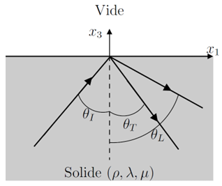
The solid is characterized by the density \(\rho\) and by the Lamé coefficients \(\lambda\) and \(\mu\). Initially, the nature of the incident wave is not defined. This wave propagates in the plane (\(\vector{x}_1\), \(\vector{x}_3\)) with an angle of incidence \(\theta_I\) and a speed \(v_I\). Its direction of propagation is represented by the vector \(n_I=(\sin{\theta_I}, 0, \cos{\theta_I})^T\). The field of movement at a point of coordinate \(\vector{r}=(x_1, x_2, x_3)^T\) representing the incident wave has the expression
- vector {u} _I (vector {r}) =vector {Q} _I e^ {-jk_ivector {n} _Icdotvector {r}}
- label:
eq:oblique1
with \(\vector{Q}_I=(Q_1,Q_2,Q_3 )^T\) and \(k_I=\frac{\omega}{v_I}\). It can be shown that three waves can exist in isotropic solids: one longitudinal wave and two transverse waves. The hypothesis is therefore made that these three waves can be generated during the interaction of the incident wave with the surface when \(x_3=0\). The reflected longitudinal wave propagates in the \(\vector{n}_L=(\sin{\theta_L}, 0, -\cos{\theta_L})^T\) direction and the two reflected transverse waves propagate in the \(\vector{n}_T=(\sin{\theta_T},0,-\cos{\theta_T})^T\) direction. Thus, the field of displacement of the reflected waves has the following expression:
- vector {u} _R (x_1, x_3) =vector {u} _L+vector {u} _ {T_1} +vector {u} _ {T_2}
- label:
eq:oblique2
with:
- left{begin {array} {ll}
vector {u} _L (vector {r}) = r_ {r}) = r_ {IL}{IL}vector {r} _Lvector {n} _Lcdotvector {r}}\ vector {u} _ {T_1} (vector {r}) = r_ {IT_1}vector {Q} _ {T_1} e^ {-jk_Tvector {n} _Tvector {n} _Tcdotvector {r}}\ vector {u} _ {T_2} (vector {r}) = r_ {IT_2}vector {Q} _ {T_2} e^ {-jk_Tvector {n} _Tvector {n} _Tcdotvector {r}} end {array}right. :label: eq:oblique3
where \(r_{IL}\), \(r_{IT_1}\) and \(r_{IT_2}\) are reflection coefficients in terms of amplitude of movement. The longitudinal displacement field is irrotational, which means that the polarization vector \(\vector{Q}_L\) is collinear to the vector \(\vector{n}_L\). Likewise, the two transverse displacement fields have zero divergence, which means that the polarization vectors \(\vector{Q}_{T_1}\) and \(\vector{Q}_{T_2}\) are orthogonal to the vector \(\vector{n}_T\). The polarization vectors therefore have the following expressions:
- left{begin {array} {ll}
vector {Q} _L= (sin {theta_L}, 0, -cos {theta_L}) ^T r_ {IL}\ vector {Q} _ {T_1} = (cos {theta_T}, 0,sin {theta_T}) ^T r_ {IT_1}\ vector {Q} _ {T_2} = (0.1.0) ^T r_ {IT_2} end {array}right. :label: eq:oblique4
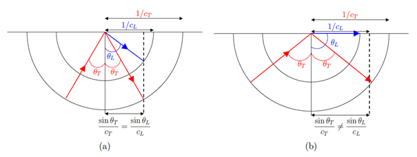
The first transverse wave is subsequently called a « transverse vertical » wave and the second is called a « transverse horizontal » wave. Taking into account the laws of Snell-Descartes, we obtain:
- sin {theta_I} /v_i =sin {theta_L} /v_L =sin {theta_T} /v_T
- label:
eq:oblique5
The move \(u=u_I+u_T\) in half-space can be written as:
- vector {u} (x_1, x_3) =f (x_1) =f (x_1)cdot (vector {Q} _I e^ {-jk_ii x_3}} +r_ {IL}}IL}vector {Q} _1)vector {Q} _L e^ {-jk_L} _I e^ {-jk_lcos {theta_I x_3}} +r_ {IT_1}vector {Q} _ {T_1} e^ {-jk_Tcos {theta_T x_3}} +r_ {IT_2}vector {Q} _ {T_2} e^ {-jk_Tcos {theta_T x_3}})
- label:
eq:oblique6
where \(f(x_1)=e^{-jk_I \sin{\theta_I}x_1 }=e^{-jk_L \sin{\theta_L}x_1 }=e^{-jk_T \sin{\theta_T}x_1 }\). In order to determine the three amplitude reflection coefficients, it is necessary to apply border conditions. These conditions are zero stress conditions at the surface (x_3=0) of the material:
- matrix {sigma}vector {e} _3 = 0Rightarrow
begin {bmatrix} sigma_ {11} &sigma_ {12} &sigma_ {13}\ sigma_ {21} &sigma_ {22} &sigma_ {23}\ sigma_ {31} &sigma_ {32} &sigma_ {33} end {bmatrix} begin {bmatrix} 0\ 0\ 1 end {bmatrix} = begin {bmatrix} 0\ 0\ 0 end {bmatrix} :label: eq:oblique7
The application of border conditions then corresponds to the following three scalar equations:
It is therefore necessary to calculate the expressions in \(x_3=0\) of the constraints \(\sigma_{13}\), \(\sigma_{23}\) and \(\sigma_{33}\) associated with each of the four waves in presence. To do this, we will use Hooke’s law:
- sigma_ {ij} =lambda (partial u_k)/(partial x_k)delta_ {ij} +mu ((partial u_i)/(partial x_j)/(partial x_j) + (partial x_j) + (partial x_i))
- label:
eq:oblique9
Therefore, using equations eq:oblique9 and eq:oblique6 we are in a position to be able to determine the constraints \(\sigma_{13}\), \(\sigma_{23}\) and \(\sigma_{33}\). The system of equations can therefore be rewritten as a system of three equations in three unknowns:
- left{begin {array} {ll}
K_lsin {(2theta_L)} r_ {L)} r_ {IL} +k_Tcos {(2theta_T)} r_ {IT_1} =K_i (cos {theta_I} Q_1+sin {theta_I} Q_3)\ K_tcos {theta_T} r_ {IT_2} = K_icos {theta_I} Q_2\ -omega Z_Lcos {2theta_T} r_ {IL} +omega Z_Tsin {2theta_T} r_ {IT_1} = K_i [lambda sin {theta_I} Q_1} Q_1 + (lambda + 2mu) cos {theta_I} Q_3 end {array}right. :label: eq:oblique10
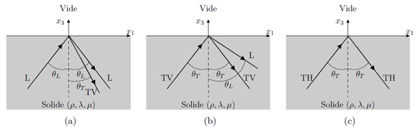
with \(Z_L=\rho v_L\) impedance associated with the longitudinal wave and \(Z_T=\rho v_T\) impedance associated with the transverse wave. It is immediately obvious that the second equation of this system is independent of the other two equations. The reflection coefficients \(r_IL\) and \(r_{IT_1}\) are independent of the component \(Q_2\) of the polarization vector of the incident wave and the reflection coefficient \(r_{IT_2}\) is independent of the components \(Q_1\) and \(Q_3\). It follows that if the incident wave is a longitudinal or vertical transverse wave, there is no reflected horizontal transverse wave (see u2.06.05-refle (a) and u2.06.05-refle (b)) and, in the same way, if the incident wave is a horizontal transverse wave, there are no reflected longitudinal and transverse vertical waves (see u2.06.05-refle (c)). In this second case, it is deduced from the second equation of the system eq:oblique10 that the reflection coefficient \(r_{IT_2}\) is equal to 1. In the following, the cases of a longitudinal incident wave and a vertical transverse incident wave are treated separately.
Longitudinal incident wave
« « » « « » « » « » « » « » « » « »
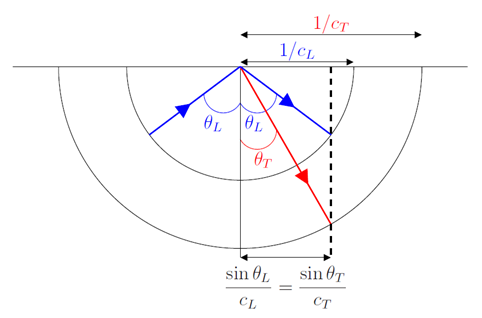
In the case of isotropic solids, the velocities of the longitudinal and transverse waves are the same in all directions. As a result, slownesses, i.e. the opposite of speeds, are also the same in all directions. The laws of Snell-Descartes can then be easily interpreted by observing the surfaces of slowness presented on u2.06.05-longitu. Reading these surfaces quickly shows that the angle \(\theta_T\) is always less than the angle of incidence \(\theta_L\) and therefore that the reflected vertical transverse waves are always propagating plane waves.
If the incident wave is a longitudinal wave, the polarization vector is collinear with vector \(\vector{n}_L\). The polarization vector is therefore of the \(\vector{Q}_L=(sin{\theta_L}, 0, cos{\theta_L})^T\) type. The first and the third equations of system eq:oblique10 can then be put into the following matrix form:
- begin {bmatrix}
kappasin {2theta_L} &cos {2theta_T}\ -cos {2theta_T} &kappasin {2theta_L} end {bmatrix} begin {bmatrix} r_ {LL}\ r_ {LT}\ end {bmatrix} = begin {bmatrix} kappasin {2theta_L}\ cos {2theta_T} end {bmatrix} :label: eq:oblique11
with \(\kappa=v_T/v_L\). The resolution of this system leads to the following expression of the reflection coefficients:
- left{begin {array} {ll}
r_ {LL} &=frac {1} {N} {N}left [kappa^2sin {2theta_L}sin {2theta_T} -cos^2 {2theta_T}right]\ r_ {LT} &=frac {2kappa} {N}sin {2theta_L}sin {2theta_T} end {array}right. :label: eq:oblique12
with \(N = \kappa^2 \sin{2\theta_L} \sin{2\theta_T} + \cos^2{2\theta_T}\).
Vertical transverse incident wave « « » « « » « » « » « » « » « » « » « » « «
The slow surfaces corresponding to an incident vertical transverse wave are shown on u2.06.05-tranv. Reading these surfaces quickly shows that angle \(\theta_T\) is always less than angle of incidence \(\theta_L\). However, when the angle \(\theta_L=90°\), the angle of incidence is equal to a critical angle \(\theta_L^c=arcsin{(v_T/v_L)}\) representing the limit between the domain of propagative reflected longitudinal waves (\(\theta_T \leq \theta_L^c\)) and the domain of evanescent reflected longitudinal waves (\(\theta_T \geq \theta_L^c\)).
If the incident wave is a vertical transverse wave, the polarization vector is perpendicular to vector \(\vector{n}_T\). The polarization vector is therefore of the \(\vector{Q}_I=(\cos(\theta_T),0,-\sin(\theta_T))^T\) type. The first and the third equations of system eq:oblique10 can then be put into the following matrix form:
- begin {bmatrix}
kappasin {2theta_L} &cos {2theta_T}\ -cos {2theta_T} &kappasin {2theta_L} end {bmatrix} begin {bmatrix} r_ {LL}\ r_ {LT}\ end {bmatrix} = begin {bmatrix} kappasin {2theta_T}\ cos {2theta_T} end {bmatrix} :label: eq:oblique13
The resolution of this system leads to the following expression of the reflection coefficients:
4.5. Usage in code_aster#
Taking into account absorbent elastic elements and calculating their impedance requires specific modeling on absorbent borders:
in 2D with the “D_ PLAN_ABSO “modeling on the absorbent edges.
in 3D with the “3D_ ABSO “modeling on the absorbent faces.
Since the formulation of these elements is fairly rudimentary to be able to precisely assimilate them to discrete shock absorbers and therefore be used in harmonic analyses, consequently, on the one hand, they should not be blocked during dynamic analyses, and on the other hand, one drawback is that the quality of their use depends on the quality of the shape of the border. A good test of this quality is inspired by test cases SDLV120 and SDLV121 and may be based on the more or less total absorption at this border of a displacement wave passage imposed at the top of the structure. As with these tests, we can ensure that the wave does not come back by looking at a speed degree of freedom on a node near the border.
In harmonic analysis with the operator DYNA_LINE_HARM [U4.53.11], mechanical damping is calculated beforehand by the option AMOR_MECA of the operator CALC_MATR_ELEM [U4.61.01] and it is entered in DYNA_LINE_HARM (keyword MATR_AMOR).
In transient analysis, the calculation of mechanical damping is automatic with the models of absorbent elements in the operator DYNA_NON_LINE [U4.53.01]. With the operator DYNA_LINE_TRAN [U4.53.02], this mechanical damping is calculated explicitly beforehand by the option AMOR_MECA of the operator CALC_MATR_ELEM [U4.61.01] and it is entered using the keyword MATR_AMOR.
For these two analyses, the calculation of the added mechanical stiffness is automatic with the models of absorbent elements when option RIGI_MECAquel is systematically calculated regardless of the calculation operator.