4.2. Thermal
The expression of the vectors \({A}^{\text{ij}}((i,j)\in {\left\{m,s,i\right\}}^{2},i\le j)\) defined in [§ 3.2.1] is obtained from the conductivities \({k}_{m}\) of the material \(m\) constituting the layers \(n\). In the cases of orthotropy \((L\text{,}T)\) of the material \(m\), the conductivity coefficients are:
(4.2)\[\begin{split} {k} _ {(L, T)}} = (\ begin {array} {c} {k} _ {L}\\ {k} _ {T}\\\ 0\ end {array})\end{split}\]
In the case of a transverse isotropic material, the coefficient \({k}_{\text{33}}\) is equal to \({k}_{T}\). To have the expression of \({A}^{\text{ij}}\) in the coordinate system of the \(({V}_{1},{V}_{2})\) element, we must apply the following rotation, from the orthotropy coordinate system to the element coordinate system, as explained in [§ 3]:
(4.3)\[\begin{split} {k} ^ {(m)} = (\ begin {array} {c} {c} {k} _ {\ text {11}}\\ {k} _ {\ text {22}}\\ {k} _ {\ text {12}}}\\ text {12}}}}\ end {12}}}\\ {12}}\\ text {12}}}\\ {12}}\\ text {12}}}\\ {12}}\\ text {12}}}\ end {array}}) = (\ begin {array}}) = (\ begin {array}} {array}) = (\ begin {array}} {cc} {C} ^ {2} & {S} ^ {2}} _ {\ text {12}}} _ {\ text {12}}}} & {C} ^ {2}\\\ text {CS} & -\ text {CS} & -\ text {CS}\ end {array}) {(\ begin {array} {c} {k} _ {L}\\ {k}\\ {k} _ {k} _ {k} _ {k} _ {k} _ {k} _ {k} _ {k} _ {k} _ {k} _ {k} _ {k} _ {k} _ {k} _ {k} _ {k} _ {k} _ {k} _ {k} _ {k} _ {\end{split}\]
The vectors \({A}^{\text{ij}}\) can then be expressed by integration into the thickness of the layer contributions:
(4.4)\[ {A} ^ {\ text {ij}} =\ sum _ {n=1} ^ {n=1} ^ {{N} _ {\ text {couch}}} {\ int} _ {3} ^ {n-1}} ^ {n-1}}}} ^ {x}}} {n} _ {3}}} ^ {x} _ {3}}} ^ {x} _ {3}}} ^ {x} _ {3}}} ^ {n}}} ^ {x} _ {3}}} ^ {x} - {n-1}}}} ^ {x} - {n-1}}}} ^ {x} - {n-1}}}} ^ {x} - {n}}} {3}} ^ {x} _ {1}}} ^ {x} - {n}}}} _ {3})\ cdot {k} _ {(m)}\ cdot {\ text {xx}} _ {3}\]
The \({B}^{\text{ij}}((i,j)\in {\left\{\mathrm{2,}3\right\}}^{2},i\le j)\) terms are:
(4.5)\[ {B} ^ {\ text {ij}} =\ sum _ {n=1} ^ {n=1} ^ {{N} _ {\ text {couch}}} {\ int} _ {3} ^ {n-1}}} ^ {n-1}}} ^ {n-1}}} ^ {n-1}}} ^ {n}} ^ {3}}} ^ {x}}} {\ partial {x}} _ {3}}\ cdot\ frac {\ partial {P} _ {p} _ {P} _ {P} _ {P} _ {3})} {\ partial {x} _ {3}}\ cdot {k} _ {\ text {k} _ {k} _ {3} _ {3} _ {3} _ {3}\]
Likewise for \({C}^{\text{ij}}\):
(4.6)\[ {C} ^ {\ text {ij}} =\ sum _ {n=1} ^ {n=1} ^ {{N} _ {\ text {couch}}} {\ int} _ {3} ^ {n-1}} ^ {n-1}}}} ^ {x}}} {n} _ {3}}} ^ {x} _ {3}}} ^ {x} _ {3}}} ^ {x} _ {3}}} ^ {n-1}}} ^ {x}}} {n}} {3}} ^ {x} _ {3}}} ^ {n}}} ^ {x} _ {3}}} ^ {x} -1}}} ^ {n-1}}} ^ {x} _ {1}}} ^ {x} _ {1}}} ^ {x}} _ {3})\ cdot {\ mathrm {\ mathrm {\ rho C}}} _ {(m)}\ cdot {\ text {xx}}} _ {3}\]
4.3. Thermomechanics
4.3.1. Behavioral relationship
In the case of laminated shells, it is shown that the relationship between the deformations \(\varepsilon\) and the stress \(\sigma\) in the layer \(n\) depends on the constants of the orthotropic material \(m\). For the elastic coefficients, we have \({E}_{\text{LL}}^{(m)}\), \({E}_{\text{TT}}^{(m)}\), \({\nu }_{\text{LT}}^{(m)}\),, \({G}_{\text{LT}}^{(m)}\),, \({G}_{\text{LZ}}^{(m)}\) and \({G}_{\text{TZ}}^{(m)}\) and the expansion coefficients \({d}_{}^{(m)}\) and \({d}_{\text{TT}}^{(m)}\). In the orthotropy axes \((L,T)\) of the material \(m\), the flexibility matrix \(S\) is expressed by:
(4.7)\[\begin{split} {S} _ {(m)} {\ mid} _ {(L, T)} _ {(L, T)}} = {\ left [\ begin {array} {ccc}}\ frac {{E} _ {\ text {LL}}}} {\ text {LL}}} {\ text {\ array}} {{E}} _ {\ mathrm {TT}} _ {\ text {LL}}}} {\ text {LL}}}} & -\ frac {LL}}}} & -\ frac {{LL}}}} & -\ frac {{\nu}} _ {\ text {\nu}} _ {\ text {\\nu}} _ {\ text {\\nu}} _ {\ text {\\nu}} _ {\ text {\ ac {{\nu} _ {\ text {TL}}}} {{E}}} {{E}} _ {\ mathrm {TT}}} &\ frac {1} {{E} _ {\ mathrm {TT}}}}}} & 0\\ 0&\ 0& 0& 0&\ 0& 0&\ 0& 0&\ frac {1} {{G}} _ {{G}} _ {{G}}}\ end {array}\ right]} _ {(m)}}\end{split}\]
Stiffness \({\Lambda }_{(m)}={S}_{(m)}^{-1}\) being:
(4.8)\[\begin{split} {\ Lambda} _ {(m)} {\ mid} _ {\ mid} _ {(L, T)} _ {\ left [\ begin {array} {ccc}}\ frac {{E} _ {\ text {LL}}}}} {\ text {LL}}}} {\ text {LL}}}}} {\ text {LL}}}}} {1- {\nu}}} {1- {\nu} _ {\ text {LL}}}}} {1- {\nu}}} {1- {\nu} _ {\ mathrm {TL}} _ {\ text {LL}}}}} {1- {\nu}}} {1- {\nu} _ {\ text {LL}}}}} {1- {\nu}}} _ {\ text {TL}}\ cdot {E}} _ {\ text {E}} _ {\ text {LL}}}} {1- {\nu} _ {\ text {LT}}} _ {\ text {LT}}}}} & 0\\\ frac {{LL}}}} {1- {\nu} _ {\ mathrm {TL}}}\ cdot {\nu}} _ {\ text {LT}}} &\ frac {{E} _ {\ mathrm {TT}}}} {1- {\nu}} _ {\ mathrm {\nu}} _ {\ text {TT}}}} {\ mathrm {TL}}}} {1- {\nu} _ {\ mathrm {TL}} _ {\ mathrm {TL}} _ {\ mathrm {TL}}} _ {\ mathrm {TL}} _ {\ mathrm {TL}} _ {\ mathrm {TL}} _ {\ mathrm {TL}} _ {\ mathrm {TL}} _ {\ mathrm {TL}} {\ text {LT}}\ end {array}\ right]} _ {(m)}\end{split}\]
For its part, transverse shear stiffness is expressed as follows:
(4.9)\[ {\ Lambda} _ {\ tau (m)} {\ mid} _ {\ mid} _ {(L, T)}}\ text {} =\ text {} {\ left [\ begin {array} {cc} {G}} _ {\ mathrm {LZ}} _ {\ mathrm {LZ}} _ {\ mathrm {LZ}}}\ end {array} {G}} _ {\ mathrm {LZ}}} _ {\ mathrm {LZ}}} _ {(m)}\]
By placing ourselves in the coordinate system of element \(({V}_{1},{V}_{2})\), we use the transition matrix \({P}^{(m)}\) from the deformation tensor defined at [§3] of \(({V}_{1},{V}_{2})\) to the orthotropy coordinate system:
(4.10)\[\begin{split} {P} ^ {(m)} =\ left [\ begin {array} {\ begin {array} {ccc} {C} {C} ^ {2} & 2\ text {CS}\\ {S} ^ {2} & {C} ^ {2} & {C} ^ {2} & {C} ^ {2} & {C} ^ {2} & {C} ^ {2} & {C} ^ {2} & {C} ^ {2} & {C} ^ {2} & {C} ^ {2} & {C} ^ {2} & {C} ^ {2} & {C} ^ {2} & {C} ^ {2} & {C} ^ {2} & {C} ^ {2} & {C} ^ {2} & {C} ^ {2} & {2}\ end {array}\ right]\end{split}\]
Likewise, the expansion vector is expressed in coordinate system \(({V}_{1},{V}_{2})\):
(4.11)\[ \begin{align}\begin{aligned}\begin{split} {d} ^ {(m)} = (\ begin {array} {c} {d} {d} _ {\ text {11}}\\ {d} _ {\ text {22}}\\ {d} _ {\ text {12}}}\\ text {12}}}\ end {12}}}\ end {array} {12}}} {\ text {12}}}\\ text {12}}}\\ {d} _ {\ text {12}}}\ end {array}}}\ end {12}}}\ end {array}} {\ text {12}}}\ end {array}}}\ end {12}}}\ end {array}} {\ text {12}}}\ end {array}}}\ end {12}}}\ end {array}}}}\\ {d} _ {\ text {TT}}}\\ 0\ end {array}})} _ {(L, T)} = (\ begin {array} {cc} {C} ^ {2} & {S} ^ {2} & {S} ^ {2}}\\ {S} ^ {2}}\\ 2\ text {CS} {2}\ text {CS} {2} & -2\ text {CS} & -2\ text {CS} & {S} ^ {2} & {S} ^ {2}\ text {CS} & -2\ text {CS} & {S} ^ {2}\ text {CS} & -2\ text {CS} & {S} ^ {2}\ text {CS} & -2\ text {CS}} & {S} ^ {2}}\) {(\ begin {array} {c} {d} _ {d} _ {LL}\\ {d} _ {\ mathrm {TT}}\ end {array})}} _ {(L, T)}\end{split}\\ So in layer :math:`n` (material: :math:`m`), in :math:`{x}_{3}`, we have:\end{aligned}\end{align} \]
(4.12)\[ {s} _ {(n)} = {P} _ {s} ^ {{} ^ {{} ^ {(m)} ^ {-1}}}}\ text {.} \ Lambda {\ mid} _ {(L, T)}\ text {.} {P} ^ {(m)}\ text {.} (e (u) - {e} ^ {\ text {th}}) = {} ^ {T}\ text {} {P} ^ {(m)}}\ text {.} \ Lambda {\ mid} _ {(L, T)}\ text {.} {P} ^ {(m)}\ text {.} (e (u) - {e} ^ {\ text {th}}) = {\ text {th}}) = {\ Lambda} _ {(m)}} (e (u) - {e}} ^ {\ text {th}}) = {\ text {th}}) = {\ text {th}})\]
With:
(4.13)\[\begin{split} \ epsilon\ left (u\ right) =\ left (\ begin {array} {c} {E} {E} _ {11}\ {E} _ {22}\\ {E} _ {12}\ end {array}\\\\\\\ right) + {x}}\\ {right) + {x} _ {right) + {x} _ {right) + {x} _ {right) + {x} _ {3}\ _ {3}\ {3}\\ {K}\ {K}} _ {12}\ end {array}\ right)\end{split}\]
Note:
In the code, we chose to perform the transition from the orthotropy coordinate system to the element coordinate system in two steps. A first step concerns the transition from the orthotropy coordinate system to the coordinate system defined by ANGL_REP. The data of DEFI_MATERIAU is thus transformed during this first pass. The equivalent material is then treated as would be done with conventional plate elements.
The treatment of thermal expansion is done in the form of a contribution to the second member of the matrix equation to be solved based on the principle of virtual work. This post reads: \({\sigma }^{{\text{th}}_{\left(n\right)}}=-{}^{T}\text{}{P}^{\left(m\right)}\text{.}\Lambda {\mid }_{\left(L,T\right)}\text{.}\left\{\begin{array}{c}{d}_{\text{LL}}\Delta T\\ {d}_{\text{TT}}\Delta T\\ 0\end{array}\right\}\).
4.3.2. Transverse shear
The transverse shear stiffness of each layer is written in coordinate system \(({V}_{1},{V}_{2})\) in the same way as the expansion:
(4.14)\[ {\ Lambda} _ {t (m)} {\ mid} _ {({V} _ {1}, {V} _ {2})} = {} ^ {t}\ text {} {P} _ {P} _ {2} _ {2} _ {2}} ^ {(m)}\ text {.} {\ Lambda} _ {t (m)}\ text {.} {P} _ {2} ^ {(m)}\]
With \({P}_{2}^{(m)}=\left[\begin{array}{cc}C& S\\ -S& C\end{array}\right]\) the vector transition matrix from \(({V}_{1},{V}_{2})\) to the orthotropy coordinate system. The overall transverse shear stiffness of the shell \(\left[{R}_{c}\right]\) calculated so as to be equal to that given by the law of three-dimensional elasticity [bib2], the matrix \(\left[{R}_{c}\right]\) is defined so that the surface density of transverse shear energy \({U}_{2}\) obtained for a three-dimensional distribution of the stresses \({\sigma }_{\text{13}}\) and \({\sigma }_{23}\) is identical to that associated with the Reissner-Mindlin plate model noted \({U}_{2}\). In the end:
(4.15)\[ {U} _ {1} =\ frac {1} {2} {2} {\ int} _ {\ int} _ {-h}\ langle\ tau\ rangle {\ left [{\ Lambda} _ {\ tau\ left (m\ left (m\ right)} {m\ right)}\ right]}\ right]} ^ {-1}\ left\ {\ tau\ right\} {d} _ {3}\]
And:
\[\]
: label: eq-50
{U} _ {2} =frac {1} {2} {2} V {left [{R} _ {c}right]} ^ {-1} V=frac {1} {2}left ({int} _ {int} _ {int} _ {int} _ {2} _ {c} _ {c}right]} ^ {-1}frac {1} {2}left ({int} _ {-h} ^ {h}left{tauright}} {d} _ {3}right)
With \(\langle \tau \rangle =\langle {\sigma }_{13}{\sigma }_{23}\rangle\). With the equilibrium equations:
(4.16)\[\begin{split} \ {\ begin {array} {c} {\ sigma} _ {\ sigma} _ {\ text {13}} _ {-h} ^ {{x} _ {3}} ({\ sigma} _ {\ text {11}\ text {11}}\ mathrm {11}}\ mathrm {11}}\\ {11}} _ {11}}\\ {sigma} _ {\ text {23}} =- {\ int} _ {\ int} _ {-h} _ {3}} ({\ sigma} _ {\ text {12}\ mathrm {,1}}} + {s}} + {s}} _ {s}} _ {s}} _ {1}} + {s}} _ {1}}} + {s}} _ {1}} + {s}} _ {1}} + {s}} _ {s}} _ {1}} + {s}} _ {s}} _ {1}} + {s}} _ {s}} _ {1}} + {s}} _ {s}} + {s}\end{split}\]
And the conditions:
\[\]
: label: eq-52
0= {sigma} _ {text {13}}} = {sigma} _ {text {23}}}
The plane stresses \({\sigma }_{11}\), \({\sigma }_{22}\) and \({\sigma }_{12}\) are expressed as a function of the resulting forces by assuming pure flexure and the absence of membrane/flexure coupling. The result is that:
(4.17)\[ \ sigma ({x} _ {3}) = {x} _ {3}\ text {.} {\ Lambda} _ {(m)} ({x} _ {3}) {P} ^ {-1}\ text {.} M\]
Where \(P\) is the flexural stiffness matrix of the entire multilayer defined by the first equation of (). These calculations, as well as the following ones, are to be performed in a single coordinate system. In Code_Aster, we choose the coordinate system intrinsic to the element. It is therefore necessary to transform the matrix A into this coordinate system. We then have:
(4.18)\[ \ left\ {\ tau ({x} _ {3})\ right\})\ right\} = {D} _ {1} ({x} _ {3}) V+ {D} _ {2} ({x} _ {3})\ left\ {\ lambda\ right\}\]
With:
(4.19)\[ \begin{align}\begin{aligned} V=\ langle {M} _ {\ mathrm {11.1}}} + {M} _ {\ mathrm {12.2}}; {M} _ {\ mathrm {12.1}}} + {M}} _ {\ mathrm {22.2}}\ rangle\\ And:\end{aligned}\end{align} \]
(4.20)\[ \ langle\ lambda\ rangle =\ langle {M} _ {\ mathrm {11.1}} - {M} _ {\ mathrm {12.2}}; {M} _ {\ mathrm {12.1}} - {M}} - {M}} _ {\ mathrm {22.2}}; {M} _ {\ mathrm {22.1}}}; {M} _ {\ mathrm {12.1}}} - {M} _ {\ mathrm {12.1}}} - {M} _ {\ mathrm {12.1}}} - {M}} thrm {11,2}}\ rangle\]
And:
(4.21)\[\begin{split} \ begin {array} {c} {D} _ {1} = {\ int} _ {\ int} _ {- {x} _ {3}} ^ {h} -\ frac {z} {2}\ left [\ begin {array} {cc} {cc} {cc} {cc} {cc}} {cc} {CC} {CC} {CC} {A} _ {\ text {13}} {cc} {cc} {CC} {A} _ {A} _ {\ text {13}} {CC} {CC} {CC} {A} _ {CC} {CC} {A} _ {\ array} {cc} {CC} {A}} = {\ text {13}} {CC} {CC} {A} = {\ array} {1} = {\ array} {1} _ {\ text {32}}\\ {A} _ {\ text {33}} _ {\ text {31}} _ {\ text {23}}} & {A} _ {\ text {22}} + {A} _ {\ text {33}}} _ {33}}} _ {\ text {33}}} _ {\ text {33}}} _ {3}}\ end {array}}} _ {33}} _ {3}}\ end {array}}} _ {3}} ^ {h} -\ frac {z} {2}\ left [\ begin {array} {\ begin {array} {cccc} {A} _ {\ text {33}} & {A}} & {A} _ {\ text {13}}}\ left [\ text {13}}}\ left [\ text {13}}}\ left [\ text {13}}}\ left [\ text {13}}}\ left [\ text {13}}}\ left [\ text {13}}}\ left [\ text {13}}}\ left [\ text {13}}}\ left [\ text {13}}}\ left [\ text {13}}}\ left [\ text {13}}}\ left [\ text {13}}\ left [\ text {13}}\ left thrm {2A}} _ {\ text {31}}}\\ {A}}\\ {A} _ {\ text {31}} _ {\ text {23}} & {A} _ {\ text {33}} - {A} - {A} _ {\ text {22}}} _ {\ text {22}}} _ {\ text {22}}} & {\ mathrm {2A}}} _ {\ text {32}} & {\ mathrm {2A}}} - {\ text {33}}} - {A}} - {A}} - {A}} - {A}} - {A}} _ {\ text {33}} - {A}} - {A}} - {A}} - {A}} - {A}} - {A}} {21}}\ end {array}\ right]\ text {dz}\ end {array}\end{split}\]
So \({U}_{1}\) is written as:
(4.22)\[ {U} _ {1} =\ frac {1} {2}\ langle V\ mid\ mid\ lambda\ rangle\ left [\ begin {array} {cc} {C} _ {\ text {11}}} & {C}} & {C}} & {C}} & {\ text {11}}} & {\ text {11}}} & {\ text {11}}} & {\ text {11}}} & {C}} & {\ text {11}}} & {C}} & {\ text {11}}} & {C}} & {\ text {11}}} & {\ text {11}}} & {C}}} & {\ text {11}}} & {C}}} & {\ text {11}}} & {C}} end {array}\ right]\ left\ {\ frac {V} {\ lambda}\ right\}\]
With:
(4.23)\[\begin{split} \ begin {array} {}\ underset {2\ times 2} {{C}} {{C}} _ {\ text {11}}}} = {\ int} _ {{h} {{D} _ {{1} ^ {T}} ^ {T}}} {\ T}}}} {\ Lambda}} _ {\ Lambda} _ {3}\\ underset} _ {3}\\ underset 2\ times 4} {{C} _ {\ text {12}}}} = {\ int}}} = {\ int} _ {\ int} _ {{1} ^ {T}} {\ Lambda} _ {\ Lambda} _ {\ tau (m)} _ {\ tau (m)}}}}}} = {\ int}}}} = {\ int} _ {1} ^ {T}}} {\ Lambda} _ {\ Lambda} _ {\ Lambda} _ {\ Lambda} _ {\ Lambda} _ {\ Lambda} _ {\ Lambda} _ {\ Lambda} _ {\ Lambda} _ {\ text {22}}} = {\ int} _ {-h} _ {-h} ^ {h} ^ {D} _ {{2} ^ {T}} {\ Lambda} _ {\ tau (m)}}}} ^ {-1}} {-1} {-1} {D} {D} _ {3}\ end {array}}}}} ^ {-1} {-1} {1} {D} {D} _ {3}\ end {array}}\end{split}\]
Hence the final trips:
(4.24)\[ {U} _ {1} = {U} _ {2}\ iff\ langle V\ mid\ lambda\ rangle\ left [\ begin {array} {cc} {C} _ {\ text {11}}} - {{H}}} - {{H} _ {c}}} - {{H} _ {H} _ {{H} _ {H} _ {H} _ {H} _ {H} _ {H} _ {H} _ {H} _ {H} _ {H} _ {H} _ {H} _ {H} _ {H} _ {H} _ {H} _ {H} _ {H} _ {H} _ {H} _ {H} _ {H} _ {H} _ {H} _ {H} _ {H} _ {H} _ {}} & {C} _ {\ text {22}}}\ end {array}\ right]\ left\ {\ frac {V} {\ lambda}\ right\} =0\ forall V,\ left\ {\ array}\ right\}\]
So we propose solution \({H}_{c}={C}_{{\text{11}}^{-1}}\). The transverse shear correction coefficients correspond to the ratio of the terms of \({H}_{c}\) to the integral over the thickness of the laminate of the terms of \({\Lambda }_{\tau (m)}\).
4.3.3. Generalized efforts
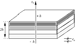
The generalized efforts put into a vector form are obtained by integration into the thickness of the shell by summing the contributions of the layers (of thickness \({e}_{n}={x}_{3}^{n}-{x}_{3}^{n-1}\)):
(4.25)\[\begin{split} \ begin {array} {c} M= (\ begin {array} {c} {c} {M} _ {\ text {11}}\\ {M} _ {\ text {22}}\\ {M} _ {\ text {12}}}\ end {12}}}\ end {12}}}\ end {array}}}\ end {array}}) = {\ int} {array}) = {\ int} _ {l}\ sigma\ cdot {x} _ {3}\ cdot {\ text {12}}} _ {3} =\ sum _ {n=1} ^ {{1} ^ {N} _ {\ text {n} _ {\ text {couch}}}} {\ int} _ {3}} ^ {x} _ {3} ^ {3} ^ {n}} {n}}} {\ n}}} {\ sigma}}} {\ sigma}} _ {\ sigma}} _ {3}\\ begin {array} {}\\ N= (\ begin {array} {c} {c} {N}} _ {\ text {11}}\\ {N} _ {\ text {22}}\\ {N} _ {\ text {12}}}\ end {12}}}\ end {array}}}\ end {array}}}\ end {array}}) = {\ end {array}}) = {\ int} {array}) = {\ int} _ {array}) = {\ int} _ {array}) = {\ int} _ {array}) = {\ int} _ {array}) = {\ int} _ {array}) = {\ int} _ {array}) = {\ int} _ {array}) = {\ int} _ {array}) = {\ int} {{N} _ {\ text {couch}}}} {\ int}} {\ int} _ {{x} _ {3} ^ {n-1}} ^ {x} _ {3} ^ {n}} {\ sigma}} {\ sigma}} _ {(n)}}\ cdot {\ text {xx}} _ {3}\ end {array} _ {3}\ end {array}\ end {n}}} {\ sigma}} _ {\ sigma}} _ {(n)} _ {3}\ end {array}} {\ sigma}} _ {\ sigma}} _ {\ sigma}} _ {\ sigma}} _ {\ sigma}} _ {\end{split}\]
If we express as before (with \(m\) material from layer \(n\)):
\[\]
: label: eq-62
{sigma} _ {(n)} = {Lambda} _ {(m)}}cdot (E+ {x} _ {3}cdot K- {d} _ {(m)}} (T ({x} _ {3})} (T ({x} _ {3})) - {T} ^ {{} _ {text {ref}}}))
We can note the widespread efforts in the form of:
(4.26)\[\begin{split} \ begin {array} {} M- {M} ^ {\ text {th}} ^ {\ text {th}} =P\ cdot K+Q\ cdot E\\ N- {N}} ^ {\ text {th}}} =Q\ cdot K+R\ cdot K+R\ cdot E\ end {array}\end{split}\]
With \(P,Q,R\) 3 x 3 matrices expressed by:
(4.27)\[\begin{split} \ begin {array} {cc} P=\ sum _ {n=1}} ^ {{n}} _ {\ text {couch}}} {\ Lambda} _ {\ int} _ {{x} _ {3} _ {3} _ {3}} ^ {n-1}}} ^ {n-1}}} ^ {3}} {x}} _ {3} ^ {2} _ {3} ^ {2} _ {3} ^ {2} _ {3} ^ {2} _ {3} ^ {2} _ {3} ^ {2} _ {3}} _ {\ x} _ {2}\ cdot {\ text {xx}}} _ {3} & =\ sum _ {n=1} ^ {n=1} ^ {1} ^ {1}} ^ {1}} ^ {3}\ cdot\ frac {1} {3}\ cdot ({({x} _ {3} _ {3} _ {3} _ {3} _ {3} {3} {3} {3} {3} {3} {3} {3}} {3} {3}}\ cdot ({x}} {3} {3} {3}} {3} {3}}\ cdot ({x}} {3} {3} {3}} {3} {3}} {3} {3}} {3} {3}}\ cdot ({x} 1}} {3} {3} {3}})\\ Q=\ sum _ {n=1} ^ {n} ^ {n} _ {\ text {couch}}} {\ Lambda} _ {(m)} {\ int} _ {{x} _ {3} ^ {n-1}}} ^ {n-1}}}} ^ {n}} _ {3}} _ {3}\ cdot {\ text {xx}} _ {3} ^ {n-1}}}} ^ {n-1}}} ^ {x}}} ^ {x}}} ^ {x} _ {3} & =\ sum _ {n=1} ^ {{N} _ {\ text {couch}}} {\ text {couch}}}} {\ Lambda} _ {(m)}\ cdot {1} {2}\ cdot ({({x} _ {3} _ {3} _ {x} _ {1}} {2})\ ({x}} _ {n-1}) {({x} _ {2})\\ R= sum\ _ {n=1} ^ {{N} _ {\ text {couch}}}} {\ Lambda} _ {(m)}\ cdot ({x} _ {3} ^ {n} _ {3} ^ {n} - {x} _ { 3} ^ {n-1}) & =\ sum _ {n=1} ^ {{n} _ {\ text {couch}}} {\ Lambda} _ {(m)}\ cdot {e}}\ cdot {e} _ {n} _ {n}\ end {array}\end{split}\]
The shear force \(V\) is obtained by deriving the moment [§ 4.3.2]. The generalized forces of thermal origin are calculated directly:
(4.28)\[\begin{split} \ begin {array} {} {M} ^ {\ text {th}} ^ {\ text {th}}} =\ sum _ {{n} _ {\ text {couch}}}} {\ Lambda}} {\ Lambda} _ {\ text {couch}}} {\ Lambda} _ {\ Lambda} _ {(m)} _ {(m)}\ text {.} {\ int} _ {{x} _ {3}} ^ {n-1}} ^ {n-1}}} ^ {3} ^ {n}} {x} _ {3} _ {3}\ text {.} (T ({x} _ {3}) - {T} ^ {\ text {ref}})\ text {.})\ text {.} {d} _ {(m)}\ text {.} {\ text {dx}} _ {3}\\ {N}} ^ {\ text {th}} ^ {\ text {th}} =\ sum _ {{n} _ {\ text {couch}}}}} {\ Lambda}} {\ Lambda} _ {(m)}\ text {.} {\ int} _ {{x} _ {3} _ {3} ^ {n-1}}} ^ {n-1}}} ^ {n-1}} ^ {3}} (T ({x} _ {3}) - {T} ^ {3}) - {T} ^ {\ text {ref}})\ text {.} {d} _ {(m)}\ text {.} {\ text {xx}} _ {3}\ end {array}\end{split}\]
4.3.4. Location of constraints (post-processing)
Conversely, following a finite element calculation and obtaining deformations \(E\) and variations in curvature \(K\), it is then possible to calculate the stress field \({\sigma }_{(n)}(n=\mathrm{1,}{N}_{\text{couch}})\) in each layer of the element.
In each layer \((n)\), it is necessary to calculate the matrix \({\Lambda }_{(m)}\) and the terms \((T({x}_{3})-{T}^{\text{réf}})\text{.}{d}_{(m)}\) (cf. [§ 3.2]) (\(m={\text{mat}}_{n}\) represents the material characteristics of the layer \(n\)).
The constraints \({\sigma }_{\alpha \beta }\) to an ordinate \({x}_{3}\in ]{x}_{3}^{n-1},{x}_{3}^{n}[\) in the layer (\(n\)) are then:
(4.29)\[ {\ sigma} _ {(n)} ({x} _ {3}) = {\ Lambda} _ {(m)}\ text {.} \ left [E+ {x} _ {3}\ text {.} K- {d} _ {(m)} (T ({x} _ {3}) - {T} _ {3}) - {T} _ {\ text {ref}}})\ right]\]
And the transverse shear:
(4.30)\[ {\ tau} _ {(n)} ({x} _ {3}) = {D} _ {3}) = {D} _ {3})\ text {.} V+ {D} _ {2} _ {2} ({x} _ {3})\ text {.} \ Lambda\]
Note:
In the code, post-treatments of plate elements are generally defined in the coordinate system associated with ANGL_REP * . The constraints in the intrinsic coordinate system of the element are thus brought back into the manifold coordinate system. We have: |
\({(\begin{array}{c}{\sigma }_{\text{11}}\\ {\sigma }_{\text{22}}\\ {\sigma }_{\text{12}}\end{array})}_{\text{eref}}=(\begin{array}{ccc}{C}^{2}& {S}^{2}& +2\text{CS}\\ {S}^{2}& {C}^{2}& -2\text{CS}\\ -\text{CS}& +\text{CS}& {C}^{2}-{S}^{2}\end{array}){(\begin{array}{c}{\sigma }_{\text{11}}\\ {\sigma }_{\text{22}}\\ {\sigma }_{\text{12}}\end{array})}_{n}\) |
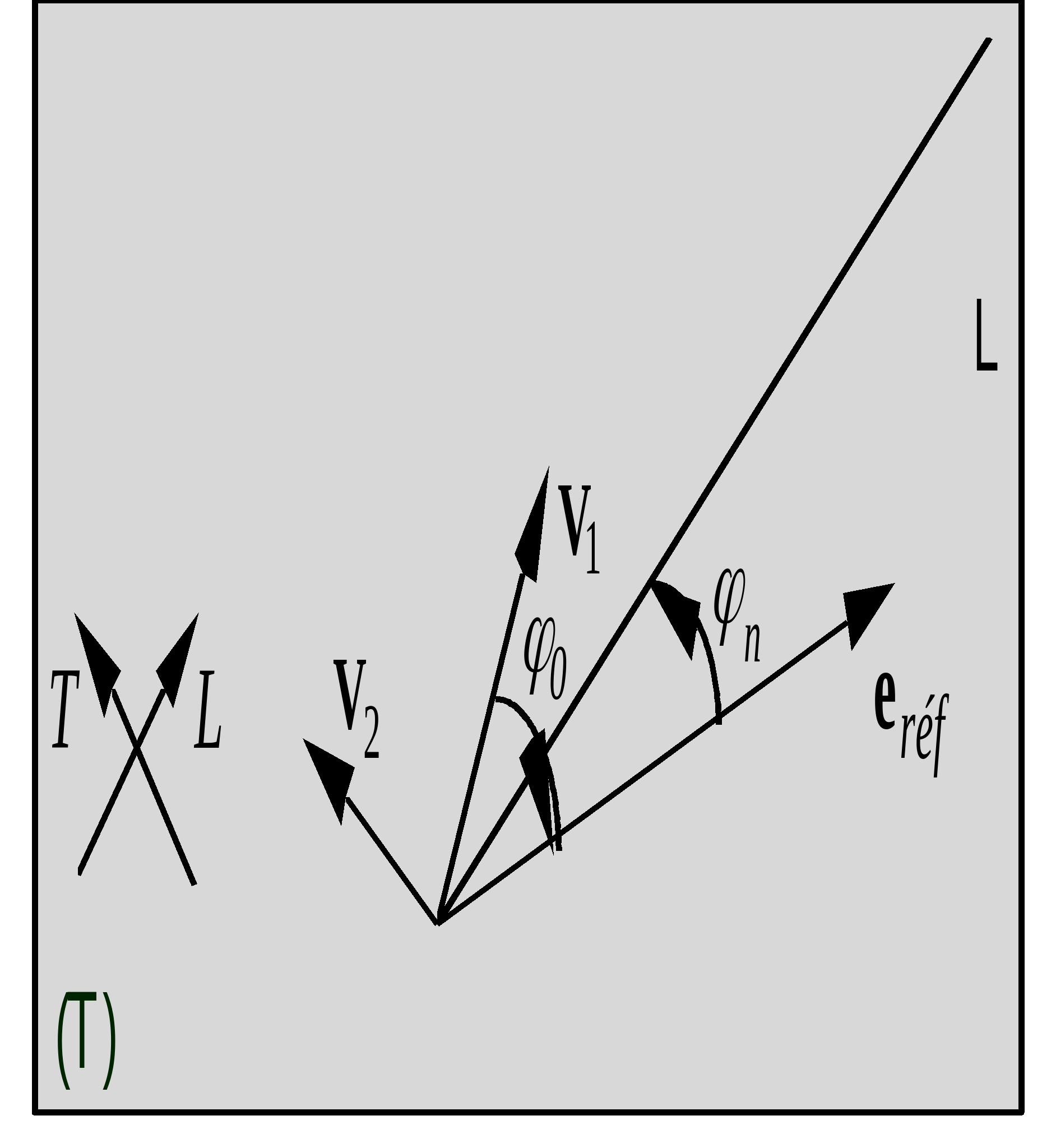
where \(\begin{array}{c}C=\text{cos}({\varphi }_{0})\\ S=\text{sin}({\varphi }_{0})\text{}(\text{cf}\text{.}\left[\S 4\text{.}1\right])\end{array}\) where \({\varphi }_{0}\) is the angle between \({V}_{1}\) and \({e}_{\text{réf}}\) |
4.3.5. Calculation of breakage criteria in diapers (post-treatment)
The breaking stress limit values depend on the material of the layer, the direction and the direction of the stress (for a group of elements corresponding to the same material field):
\(\begin{array}{}\begin{array}{ccc}\begin{array}{c}{\text{mat}}_{n}\end{array}& \begin{array}{c}X\text{: limite en traction dans le sens L}\\ {X}^{\text{'}}\text{: limite en compression dans le sens L}\\ Y\text{: limite en traction dans le sens T}\\ {Y}^{\text{'}}\text{: limite en compression dans le sens T}\\ S\text{: limite en cisaillement dans le sens LT}\end{array}& \begin{array}{c}(\text{1ère direction orthotropie : sens des fibres})\\ (\text{1ère direction orthotropie : sens des fibres})\\ (\text{2ème direction orthogonale à la 1 ère})\\ (\text{2ème direction orthogonale à la 1 ère})\\ \end{array}\end{array}\\ \end{array}\)
It is necessary to calculate the stresses in the layer coordinate system (defined by the orthotropy axes) from the constraints in the element coordinate system. The angle between \({V}_{1}\) and \({e}_{\text{réf}}\) is \({\varphi }_{0}\), and the angle between \({e}_{\text{réf}}\) and the orthotropy coordinate system is \({\varphi }_{n}\):
(4.31)\[\begin{split} {\ left (\ begin {array} {c} {\ sigma} _ {\ sigma} _ {L}\\ {\ sigma} _ {T}\\ {array}\ right)} _ {n} =\ left (\ begin {array} {\ sigma} =\ left (\ begin {array} {sigma} _ {sigma} _ {2} _ {array}\ {n} =\ {n} =\ left (\ begin {array}} {sigma} _ {n} =\ left (\ begin {array}} {sigma} _ {n} =\ left (\ begin {array}} {sigma} _ {n} =\ left (\ begin {array}} {sigma} _ {n} =\ left (\ begin {array}} {sigma} _ {n} =\ left (\ begin {array} {sigma} 2} & {C} ^ {2} & -2\ text {CS}\\ -\ -\ text {CS} & +\ text {CS} & {C} ^ {2} - {S} ^ {2}\ end {array}\\ right) {\ right) {\ left) {\ left) {\ left (\ left (\ begin {array}}\ {array} {\ array}\ right) {\ left (\ begin {array} {\ array}\ right) {\ left (\ begin {array} {c} {c}} {\ sigma}} _ {\ text {22}}\ right) {\ text {22}}\ right) {\ left (\ begin {array}}\\ {\ sigma} _ {\ text {12}}}\ end {array}\ right)} _ {n}\end{split}\]
For the maximum stress criterion, the following five criteria are calculated per layer:
(4.32)\[ \ textrm {For}
n=\ mathrm {1,} N-\ text {couch}\]
The Tsai-Hill criterion is written in each layer as follows:
(4.33)\[ {C} _ {\ text {TH}}} =\ frac {{\ sigma} _ {L (n)} ^ {2}} {{X} _ {({\ text {mat}} _ {n})} _ {n})}}} ^ {n})}} ^ {2}}} -\ frac {{\ sigma} _ {L (n)\ text {.}} {\ sigma} _ {T (n)}} {{X} _ {{X} _ {({\ text {mat}}} _ {n})} ^ {2}}\ frac {{\ sigma} _ {T (n)} _ {T (n)}} ^ {2}} _ {2}} _ {n}}\ frac {{\ sigma} _ {\ text {LT} (n)}} ^ {2}} {{S} _ {({\ text {mat}}} _ {n})}} ^ {2}}\]
The material is broken when \({C}_{\text{TH}}\ge 1\). The values \(X\) and \(Y\) are replaced by \({X}^{\text{'}}\) and \({Y}^{\text{'}}\) when the corresponding \(({\sigma }_{L(n)}\text{,}{\sigma }_{T(n)})\) constraints are negative.