4. Theoretical description of the element#
4.1. Displacement field and associated deformation field#
4.1.1. Hypotheses about kinematics#
The girder kinematics adopted is as follows:
The beam element is assumed to be straight, the cross section constant.
The cross section is undeformable in its plane but can warp axially
Transverse shear deformations are not overlooked and cause the section to rotate around its axes
Deformations are small, but displacements and rotations can be large
We place ourselves at the level of a finite element, that is to say a segment with 2 nodes. A coordinate system local to the element is defined by the axis of the segment and the main axes of geometric inertia. The center \(O\) of the coordinate system coincides with node 1 (which is the center of gravity of the section), we also define the center of torsion (or shear) \(C\) of the section, where the application of a shear force does not generate torsional work and vice versa.
It is easy to show that if the axial displacements are expressed from the displacements of point \(O\) and the displacements in the plane of the section from those of point \(C\) then all the efforts are decoupled, that is to say that the behavior matrix (for the beam elements, this is the matrix obtained after expression of Hooke’s law and integration on the section) is diagonal. The retrieval in the global frame of reference is then done in two stages: passage of all the movements in the local reference frame of center \(O\) then passage from the local frame of reference to the global frame of reference.
4.1.2. Expression of the displacement field#
For such a section, the displacement of a point \(P\) with an abscissa \(x\), with coordinates \((y,z)\) in the coordinate system \(O\) is expressed as the sum of a translation term and a rotation term (hypothesis of undeformable straight sections).
To take account of the warping of the sections, a term of non-uniform axial displacement is added. The displacement field \(\overrightarrow{\xi }\) is then written:
\(\overrightarrow{\xi }(x,y,z)=\{\begin{array}{ccc}u(x,y,z)& \text{=}& {u}_{O}(x)+(z\times {\theta }_{y}(x))-(y\times {\theta }_{z}(x))+(\omega (y,z)\times {\theta }_{x,x}(x))\\ v(x,y,z)& \text{=}& {v}_{C}(x)-((z-{z}_{C})\times {\theta }_{x}(x))\\ w(x,y,z)& \text{=}& {w}_{C}(x)+((y-{y}_{C})\times {\theta }_{x}(x))\end{array}\) |
The indices \(C\) refer to the center of torsion \(C\) which is not confused with the center of gravity \(O\) in the case of non-bi-symmetric sections. The transition from trips in \(C\) to those in \(O\) is carried out by a simple change of reference. Function \(\omega\), commonly called warpage function, and which only depends on the shape of the section, makes it possible to describe non-uniform axial displacement. The degrees of freedom of the element are carried to the nodes and are interpolated into the length of the element. There are 14 degrees of freedom, 7 at each node which are: \((u,v,w,{\theta }_{x},{\theta }_{y},{\theta }_{z},{\theta }_{x,x})\). We naturally find 3 degrees of translation and 3 degrees of rotation to describe the kinematics, in addition, the torsional rate \({\theta }_{x,x}\) is also taken as a measure of warpage.
When the rotations can no longer be considered small, it is then necessary to enrich the displacement field with a non-linear term. In fact, within the term of warping and placing itself in the center coordinate system \(O\) * , the expression () can be written vectorally as:
++—————————————————————————————————————–+———-+ ||:math:`overrightarrow{xi }(x,y,z)=overrightarrow{{xi }_{O}}(x)+(R(x)-I)(begin{array}{}0\ y\ zend{array})`|**eq** 4-2| ++—————————————————————————————————————–+———-+
This expression brings up the rotation operator \(R\). If \(P\) is the coordinate point \((y,z)\) then \(R\) makes it possible to take the vector \(\overrightarrow{\mathrm{OP}}\) into its final configuration \(\overrightarrow{\mathrm{OP}\text{'}}\). \(R\) depends on the antisymmetric matrix associated with the rotation vector \(\overrightarrow{\theta }={}^{t}({\theta }_{x},{\theta }_{y},{\theta }_{z})\) which is an unknown of the problem in the same way as \(\overrightarrow{{\xi }_{O}}\), we can even show that \(R\) is written as a matrix exponential:
\(R={e}^{\theta }=I+\theta +\frac{{(\theta )}^{2}}{2!}+\cdots +\frac{{(\theta )}^{p}}{p!}+\cdots \text{avec}\theta =(\begin{array}{ccc}0& -{\theta }_{z}& {\theta }_{y}\\ {\theta }_{z}& 0& -{\theta }_{x}\\ -{\theta }_{y}& {\theta }_{x}& 0\end{array})\) |
eq 4-3 |
- In (), this operator was replaced by its first-order development because the rotations were small. To take into account large rotations, one of the possibilities [5] _
is to develop the rotation operator at least up to the second order. We then speak of moderate rotations (finite rotations in English). It is the accumulation of these moderate rotations that will lead to large rotations.
The displacement field is then enriched with a non-linear, quadratic term in \({\theta }_{x},{\theta }_{y},{\theta }_{z}\). Second order expansion is obtained by expanding the exponential to the term in \({\theta }^{2}\).
4.1.3. Associated deformation field#
In addition, let’s calculate the Green-Lagrange deformations of the displacement field (), we already use the hypothesis of small deformations, in fact let’s consider the complete expression of Green-Lagrange deformations (since the sections are supposed to be undeformable in their plane, half of the terms are already zero):
: label: EQ-None
F=I+frac {partialoverrightarrow {xi}} {partialoverrightarrow {x}} =I+nablaoverrightarrow {xi}} =I+nablaoverrightarrow {xi}
: label: EQ-None
E=frac {1} {2} ({} ^ {t}mathrm {FF} -I) ={begin {array} {ccc} {E} _ {mathrm {xx}}} &text {=}}} &text {=} {{t}} & {u} & {u} & {u}} + {, x}} + {, x}} ^ {2} + {{v} _ {, x}} ^ {2} + {{w} _ {, x}}} ^ {2})\ 2 {E} _ {mathrm {xy}} &text {=} & ({=}} & ({u} _ {, y} + {, y}} + {, y} _ {, y} + {, y} _ {, y} + {, y} + {, y} + {, y} + {, y} + {, y} + {, y} + {, y} + {, y} + {, y} + {, y} + {, y} + {, y} + {, y} + {, y} + {, y} + {, y} + {, y} + {, y} + {, y} + {, x} {w} _ {, y})\ 2 {E})\ 2 {E} _ {mathrm {xz}}} &text {=} & ({u} _ {, z} + {w} _ {, x}}) + ({u} {, x} {, x} {, x} {, x} {, x} _ {, x}}) + ({u} _ {, x}) + ({u} _ {, x}) + ({u} _ {, x}) + ({u} _ {, x}) + ({u} _ {, x}) + ({u} _ {, x}) + ({u} _ {, x}}) + ({u} _ {, x}}) + ({u}}
Since the deformations are small, we deduce only \(∣{u}_{,x}∣\ll 1\) and therefore \(∣{u}_{,x}{u}_{,y}∣\ll ∣{u}_{,y}∣\) and \(∣{u}_{,x}{u}_{,z}∣\ll ∣{u}_{,z}∣\). We can therefore simplify the complete expression for \(E\) by neglecting the quadratic terms in \(∣{u}_{,i}∣\) or \(i=(x,y,z)\). In these terms are not overlooked, they then lead to a more complex tangent matrix expression and improved convergence. On the other hand, they do not change the precision of the results.
By injecting the displacement field () into this simplified expression we finally get the following form \(E=\epsilon +\eta\):
: label: EQ-None
epsilon ={begin {array} {ccc} {epsilon} {epsilon} _ {mathrm {xx}} &text {=} & {u} _ {O, x} (x) + (ztimes {theta}) + (ztimes {theta} (x) + (z, x} (x)) + (ztimes {theta} (x)) + (ztimes {theta}} + (ztimes {theta}} (x)) + (ztimes {theta}} + (ztimes {theta}} (x)) + (ztimes {theta}} (x)) + (ztimes {theta}} (x)) + (z(y, z)times {theta} _ {x,mathrm {xx}} (x))\ 2 {epsilon} _ {mathrm {xy}} &text {=} & ({v}}} & ({v} _ {}}) & ({v} _ {=}} & ({v} _ {=}} & (v} _ {=}} & (v} _ {}}} & (v} _ {=}} & (v} _ {}}} & (v} _ {=}} & (v} _ {}}} & (v} _ {=}} & (v} _ {}}) & ({v} _ {=}} & (v} _ {}}) & ({v} _ {=}}} _ {C})times {theta} _ {x, x} (x))\ 2 {epsilon} _ {mathrm {xz}} &text {=} & ({w} _ {C, x} (x) _ {C, x} (x) + {theta}} (x) + ({theta}} _ {y}) + (y- {y} _ {C} _ {C}) + (y- {y} _ {C} _ {C})times {theta} _ {x, x} (x))end {array}
: label: EQ-None
eta ={begin {array} {ccc} {ccc} {eta}} {eta}} _ {mathit {xx}}} &frac {1} {2} ({{v} _ {C, x}}}} ^ {x}}} ^ {x}}} +left ({(y- {y}} _ {C}}}}} ^ {C}}} ^ {2})} ^ {2})} ^ {2})} ^ {2}} + {(z- {z} _ {C})} ^ {2}right) {{theta} _ {x, x}} ^ {2}\ & +2 (y- {y} _ {C}) {theta}) {theta}) {theta}} {C}) {theta} _ {C}) {theta} _ {C}) {theta} _ {C}) {theta} _ {C}) {theta} _ {C}) {theta} _ {C}) {theta} _ {C}) {theta} _ {C}) {theta} _ {C}) {theta} _ {C}) {theta} _ {C}) {theta}, x} {v} _ {C, x})\ 2 {eta})\ 2 {eta} _ {eta} _ {x})left ({w} _ {C, x})left ({w} _ {C, x}) + (y- {y}} _ {C}) {theta} _ {C}) {theta} _ {C}) {theta} (x)right)\ 2 {eta} _ {right)\ 2 {eta} _ {mathit {xz}} &text {=} & - {theta} & - {theta} _ {x}left ({v} _ {C} - (z- {z} _ {C}) {theta}) {theta}} _ {theta} _ {x, x} (x)right)end {array}) {theta} _ {C}) {theta} _ {c}) {theta} _ {c}) {theta} _ {c}}
where \(\epsilon\) are the linearized deformations and \(\eta\) the so-called nonlinear deformations (resulting from quadratic terms in the Green-Lagrange deformations). If the nonlinear displacement field is injected for the treatment of large rotations then, an additional nonlinear term \({\eta }_{\mathrm{gr}}\) appears.
4.2. Principle of virtual work#
4.2.1. The hypotheses used#
To write the principle of virtual work (PTV), we will hypothesize a Lagrangian Formulation Updated at each Iteration (FLAI), that is to say that the geometry of the structure studied will be constantly updated. Locally, this results in the position of the nodes of the element, which changes at each iteration of the Newton algorithm, making it possible to calculate a new matrix for the transition from the local coordinate system to the global coordinate system.
- Let it be an element in initial configuration \({C}_{0}\). We can describe the deformations of the element from 3 configurations, the initial configuration
so, as well as 2 other configurations: \({C}_{1}\) which designates a deformed configuration known but not necessarily in balance and \({C}_{2}\) which designates an unknown deformed configuration close to \({C}_{1}\). The last known configuration is taken as a reference, we will write PTV in this configuration.
To locate ourselves in the resolution algorithm, we can for example imagine that \({C}_{0}\) designates the configuration at the beginning of the \((t=0)\) time steps. In addition, we have already performed a first iteration, so we have determined \({C}_{1}\) which is not in balance. We will therefore carry out a new iteration, choosing \({C}_{1}\) as a reference and writing PTV in an unknown configuration and so on… until we find a configuration in balance and then move on to the next step of time.
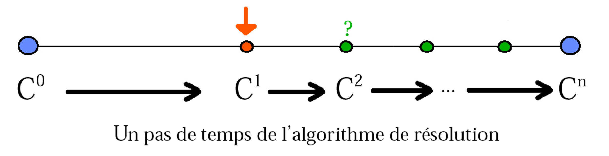
Figure 4.1: The various reference configurations.
A first remark can be made: the supports of the beam elements in the Code_Aster are segments with two nodes (SEG2), so their geometric interpolation functions are linear. With these elements, it will therefore never be possible to reproduce exactly the « last known configuration », this represents an approximation and care must therefore be taken to have a sufficiently fine mesh for problems where the curvature of the elements becomes not negligible. The solution, which consists in correcting the residue or using a co-rotational formulation, was not implemented because it would have required profound changes to the code. .
FLAI has many advantages, for example we can confuse Cauchy stress tensor (expressed on the final configuration at the previous iteration) and Piola-Kirchoff stress tensor of the second kind (expressed on the initial configuration at the current iteration) because between the two iterations, the geometry will have been updated:
: label: EQ-None
S=mathrm {det} (F) {F} ^ {-1}sigma {{} ^ {t} F} ^ {-1} =sigma
This means that in the reference configuration (the configuration in particular that allows the virtual deformations to be expressed) the initial displacements already acquired by the element will always be zero because the last calculated configuration will be taken as a reference. In general, only the initial stress state in a given configuration will be non-zero.
As far as behavior is concerned, it is written incrementally and it is expressed in Lagrangian quantities thanks to the Piola-Kirchhoff tensor \(\mathrm{II}S\) and to the Green-Lagrange deformations \(E\). The small deformations make it possible to linearize the law of behavior and therefore:
: label: EQ-None
Delta S= C:Delta Eapprox C:DeltaEpsilon
For beam elements, plane stresses in the section are assumed. This is equivalent to assuming that the beam consists of longitudinal fibers working in traction-compression.
This hypothesis (\({\sigma }_{\mathrm{yy}}={\sigma }_{\mathrm{zz}}={\sigma }_{\mathrm{yz}}=0\)) makes it possible to express the law of behavior in the case of beams in the form:
: label: EQ-None
C:Deltaepsilon ={begin {array} {c} {c} Edelta {epsilon} _ {mathrm {xx}}\ mathrm {2G}delta {epsilon} _ {mathrm {xy}} _ {mathrm {xy}} _ {mathrm {xz}} _ {mathrm {xz}} _ {mathrm {xz}} _ {mathrm {xz}} _ {mathrm {xz}} _ {mathrm {xz}} _ {mathrm {xz}} _ {mathrm {xz}} _ {mathrm {xz}} _ {mathrm {xz}} _ {mathrm
Finally, the hypothesis of a field of movement with moderate rotations will be legitimate to obtain large rotations between steps and for the total load. In fact, FLAI means that the increases in calculated movements and constraints will be summed up at the beginning of a step and at the end of each iteration. The total increase in displacement and rotation over one step may therefore be large.
4.2.2. Writing PTV and differentiating#
The principle of virtual work, which is the weak formulation of the laws of the mechanics of continuous media, is written as:
: label: EQ-None
{int} _ {{C} _ {2}}}sigma: {epsilon}} ^ {text {*}}mathrm {dV} = {int} _ {{C} _ {2}}overrightarrow {f}mathrm {.} overrightarrow {{xi} ^ {text {*}}}}mathrm {dV} + {int} _ {partial {C} _ {2}}overrightarrow {2}}overrightarrow {t}mathrm {.} overrightarrow {{xi} ^ {text {*}}}}mathrm {dS}}
where all quantities are expressed on the unknown deformed configuration, \(\sigma\) is the Cauchy stress tensor. In addition \(\overrightarrow{{\xi }^{\text{*}}}\) refers to a virtual field of movement that is kinematically admissible in the sense of boundary conditions.
To solve such a problem, one must first change the configuration by changing the variable. The principle of virtual works written in Lagrangian quantities (in the reference configuration therefore and not in the deformed configuration) is expressed using virtual Green-Lagrange deformations \({E}^{\text{*}}\) and the Piola-Kirchhoff stress tensor of the second kind (PKII) :math:`S`** . **
: label: EQ-None
{W} _ {text {int}} = {int}} = {int} _ {{int}} _ {1}} S: {E} ^ {text {*}}mathrm {dV} = {int} = {int} _ {{}} _ {C} _ {1}}overrightarrow {f}}mathrm {dV} = {int} _ {int} _ {C} _ {1}}overrightarrow {f}mathrm {dV} = {int} _ {int} _ {C} _ {1}} overrightarrow {{xi} ^ {text {*}}}}mathrm {dV} + {int} _ {partial {C} _ {1}}overrightarrow {1}}overrightarrow {t}mathrm {.} overrightarrow {{xi} ^ {text {*}}}}mathrm {dS}}
where \(\overrightarrow{f}\) represents the volume force density, \(\overrightarrow{t}\) the surface force density. Subsequently, we will note \({W}_{\mathrm{ext}}\) the right-hand side, and we will assume that the load is conservative and not consecutive so that the work of external forces is constant over a time step.
The stress tensor PKII () expresses the same quantity as the Cauchy stress tensor but taking the initial configuration as a reference. The Green-Lagrange virtual strain tensor is written as:
: label: EQ-None
{begin {array} {cccc} & {E}} ^ {E} ^ {text {*}}} &text {=} &frac {1} {2} ({} ^ {t} {F} ^ {F} ^ {F} ^ {F} ^ {F} ^ {F} ^ {F} ^ {F} ^ {F} ^ {F} ^ {F} ^ {F} ^ {F} ^ {F} ^ {F} ^ {F} ^ {F} ^ {text {*}} ^ {F} ^ {text {*}} ^ {F} ^ {text {*}} ^ {text {*}} ^ {text {*}} ^ {text {*}} ^ {text {*}} ^ {text {*}} text {=} & I+frac {partialoverrightarrow {partialoverrightarrow {{tarrow {x}}}} {partialoverrightarrow {x}}\ text {and}} & {F}} & {F}} ^ {F} ^ {F} ^ {F} ^ {text {*}} ^ {text {*}}}} {partialoverrightarrow {x}}}} {partialoverrightarrow {x}}}\text {x}}} {partialtext {x}}} {partialtext {x}}}\text {x}}} {partialtext {x}}} {partialtext {x}}}\text {and}*}}}} {partialoverrightarrow {x}}end {array}
To solve the balance one must check () for any virtual displacement kinematically admissible at zero \(\overrightarrow{{\xi }^{\text{*}}}\). We apply Newton’s method to the functional \({W}_{\text{int}}-{W}_{\mathrm{ext}}\) and to do this we differentiate the functional with respect to the unknown \(\overrightarrow{\xi }\), this makes it possible to transform the resolution of a non-linear problem (\({W}_{\text{int}}\) does not depend linearly on \(\overrightarrow{\xi }\)) into a sequence of solving linear systems.
So we solve:
: label: EQ-None
{W} _ {mathrm {ext}} = {W}} = {W} _ {text {int}}} ^ {1}} + {int} _ {1}} (Delta S: {E}} ^ {text {*}} ^ {text {*}}})mathrm {dV}} (Delta S: {E} ^ {E}}})mathrm {dV}} S:Delta
where \({W}_{\text{int}}^{1}\) represents the work already balanced in configuration 1. The principle is to balance this work with that of internal forces \({W}_{\mathrm{ext}}\) through successive iterations.
The first term under the integral models material stiffness. Indeed, as the law of behavior is linearized and since the reference configuration is the last known configuration (so \(\overrightarrow{\xi }=\overrightarrow{0}\)). ), we can write using () and ():
: label: EQ-None
{E} ^ {text {*}}} = {epsilon}} ^ {text {*}} =frac {1} {2} ({} ^ {t} {F} {F} ^ {text {*}}} +F)
: label: EQ-None
{int} _ {{C} _ {1}}}Delta S: {E}}}Delta S: {E}} ^ {text {*}}mathrm {*} _ {1}}DeltaEpsilon:C: {epsilon:C: {epsilon} ^ {text {*}}}mathrm {dV}}mathrm {dV}}
FLAI actually makes it possible here to avoid an additional term that combines non-linear virtual deformations and linear deformations and that is called the initial displacement term (these displacements are the displacements already undergone by our structure with respect to its reference configuration and which are always zero here). In fact, thanks to FLAI, we deport the change in geometry and the resulting nonlinearity into the local-global coordinate system change specific to the finite element method.
The second term under the integral models the geometric rigidity of the structure. It is thanks to this term that we will be able to translate the effects of the second order and converge quickly towards the solution. This term in fact directly involves non-linear deformations since according to (), \(\Delta {E}^{\text{*}}=\Delta {\eta }^{\text{*}}\). If the displacement field also contains non-linear terms to take into account moderate rotations, then of course, the nonlinear deformations also contain an additional term.
It remains to be noted that the Cauchy stress tensor and the PKII stress tensor are identified because the initial and final configurations are confused following the update.
4.2.3. Balance sheet#
So we have:
: label: EQ-None
Delta W= {int} _ {{C} _ {1}}} (DeltaEpsilon:C: {epsilon} ^ {text {*}}} +sigma:Delta {eta}} ^ {eta} ^ {text} ^ {text {*}} ^ {text {*}}})mathrm {*}}})mathrm {*}}})mathrm {*}})mathrm {*}})mathrm {*}})mathrm {*}})mathrm {*}})mathrm {*}})mathrm {*}})mathrm {*}})mathrm {*}})mathrm {*}}} ^ {1}
Physically, everything happens as if the residue \({W}_{\mathrm{ext}}-{W}_{\text{int}}^{1}\) is dissipated iteration after iteration by a \(\Delta W\) work partly due to the deformation of the material (material stiffness) and partly due to the large displacements of the structure (geometric rigidity). Geometric rigidity makes sense when the structure undergoes large displacements.
The term material stiffness is a classical term that is already present in the current formulation of elements POU_D_TGM. It can possibly translate material non-linearity (plasticity for example) through the multi-fiber approach.
The term geometric rigidity that is usually found in large displacements is new (in the updated reference configuration, there is generally a non-zero stress state). It therefore reflects geometric non-linearity and it is thanks, among other things, to this term omitted in formulation PETIT_REAC that convergence will be faster or even finally possible in the case of instabilities.
The second term in the right-hand side is the work of the internal forces in the previous iteration, it is its exact calculation that guarantees convergence towards a fair result, which is why, we will propose an improvement in its calculation.
It should be noted that in the term of geometric rigidity the unknown intervenes through virtual deformations, in fact the latter depend linearly on the unknowns.
4.3. Determining the tangent matrix#
4.3.1. Reminder on discretization#
Now it is a question of determining the tangent matrix, which is the combination of the various terms mentioned above. To do this, it is necessary to involve discretization in finite elements, in particular interpolation functions, and then to explain the volume integrals that intervene in ().
For structural elements such as beams, this discretization is carried out in two stages: on the one hand the integration on the sections located at the Gauss points and on the other hand the integration into the length. As a multi-fiber behavior was chosen for the treatment of plasticity, integration into the section is made thanks to the fibers for axial behavior (normal force, bending moments) and using laws of behavior under generalized efforts for the rest of the efforts.
Integrals on the section at each Gauss point (of the beam element) are calculated because it is the quantities at these points that will then allow numerical integration into the length (using Gauss quadrature formulas). The generalized deformations are then expressed using a matrix of interpolation functions. Numerical integration then makes it possible to determine a tangent matrix: we will therefore only seek here to express the matrix after integration on the section because it is its expression that will be necessary for implementation in the code, the numerical integration being transparent.
4.3.2. Expression of material stiffness#
We can explain the term material stiffness, by first explaining the law of behavior () then by replacing the linearized deformations \(\epsilon\) by their expression () and finally by integrating over the section, thus maintaining only a length integral.
: label: EQ-None
begin {array} {ccc} {int} _ {{C} _ {1}}DeltaEpsilon:C: {epsilon} ^ {text {*}}mathrm {dV} &text {dV} &text {=} & {=}} & {int} & {int} _ {int} _ {epsilon}} _ {mathrm {xx}}} {epsilon} _ {mathrm {xx}}} ^ {text {*}}} +mathrm {2G}delta {epsilon} _ {mathrm {xy}} {epsilon}} {epsilon}} _ {epsilon}} _ {epsilon} _ {mathrm {xz}} {epsilon} _ {mathrm {xz}}} ^ {text {*}})mathrm {dV}\ &text {=} & {int} & {int} & {int} _ {int} _ {int} _ {s} & {int} _ {s} & {int} _ {D} _ {D} _ {D} _ {s} ^ {text {*}}})mathrm {dl}end {array}
where we have: \({D}_{s}=BU\), \(B\) being the interpolation matrix of generalized deformations \(({u}_{O,x},({v}_{C,x}-{\theta }_{z}),({w}_{C,x}+{\theta }_{y}),{\theta }_{x,x},{\theta }_{y,x},{\theta }_{z,x},{\theta }_{x,\mathrm{xx}})\) and \(U\) being the vector of nodal unknowns.
\({K}_{s}\) is a behavioral matrix that reflects both the characteristics of the material and the geometric characteristics of the section (hence the appearance of the constants \({S}_{y}^{\text{'}},{S}_{z}^{\text{'}},J\) and \({I}_{\omega }\) referring respectively to the reduced sections, to the torsional constant and to the warping constant):
: label: EQ-None
{K} _ {s} = (begin {array} {ccccc} {ccccc} {int} _ {S} Emathrm {ds} & 0& 0& {int} _ {S}mathrm {Ez}mathrm {Ez}mathrm {Ez}mathrm {Ez}mathrm {Ez}\}\}\ mathrm {GS}} _ {y} ^ {text {“}} {text {“}} & 0& 0& 0& 0& 0\ & & {mathrm {GS}} _ {z} ^ {text {“}}}} & 0& 0& 0& 0& 0& 0\& {text {“}}} ^ {text {“}}}}} & 0& 0& 0& 0& 0\ & {text {“}}} ^ {text {“}}}}} & 0& 0& 0& 0\ & {text {“}}} ^ {text {“}}}} & 0& 0& 0& 0\& & {text {”} “}}}} & 0& 0& 0&} {mathrm {Ez}} ^ {2}mathrm {ds} & - {int} _ {S}mathrm {Ez}mathrm {ds} & 0\ &mathrm {sym} {sym} &mathrm {sym}} & & & {int} _ {S} {mathrm {Ez}} ^ {2}mathrm {ds} & 0\ & & & & & & & {mathrm {EI}}} _ {omega}end {array})
: label: EQ-None
begin {array} {ccc} {phi} _ {1} _ {1} &text {=} & {xi} _ {mathrm {1,} x} + {xi} _ {5}\ {phi} _ {5}\ phi} _ {phi} _ {phi} _ {2}phi} _ {2}phi} _ {2}phi} _ {2}phi} _ {2} _ {2}phi} _ {2}phi} _ {2}\ phi} _ {3} &text {=} & {xi} & {xi} _ {mathrm {3,} x} + {xi} _ {7}\ {phi} _ {4} &text {=} &text {=}} & - {xi}} & {xi}} + {xi} _ {4} _ {4} &text {=}}} &text {=}}} & - {xi}} + {xi} _ {4} &text {=}}} &text {=}}} & - {xi}}} + {xi} _ {8}text {=}} &text {=}}} & - { begin {array} {ccc} {psi} _ {1} _ {1} &text {=} & {xi} _ {mathrm {1,} x} - {xi} _ {5}\ {psi} _ {psi} _ {2} _ {2}} &text {=} & {xi} _ {6}{psi} _ {6}{psi} _ {2} _ {6}\ {psi} _ {2}} _ {6}\ {psi} _ {2}} _ {6}\ {psi} _ {6}{psi} _ {2}{psi} _ {6}\ {psi} _ {6}\ {psi} _ {6}\ {psi} _ {3} &text {=} & {xi} & {xi} _ {mathrm {3,} x} - {xi} _ {7}{psi} _ {4} &text {=} &text {=}} & {xi}} & {xi}} - {xi} _ {4}} _ {4}text {=}} &text {=}} & {=}} & {xi}} & {=}} & {xi}} - {xi} _ {4} &text {=}}} & {=}} & {=}} & {xi}} &text {=}} & {=}}
The surface integrals that still appear in the expression for \({K}_{s}\) refer to terms calculated using the mesh of the fiber cross section. Except in the elastic case, extra-diagonal terms are generally not zero because Young’s modulus \(E\) is then no longer homogeneous in the section.
Expressions for interpolation functions \({\xi }_{i=(\mathrm{1,}\dots ,8)},{N}_{j=(\mathrm{1,}\dots ,4)}\) are given in.
It should be noted that the approach chosen to determine the material stiffness matrix is not the one adopted in the Code_Aster for the Euler POU_D_E and Timoshenko POU_D_T beam elements. Indeed, in our work, the approach is derived from the laws of the mechanics of 3D continuous media and we give ourselves a 3D field of displacement for this, which allows us to involve large displacements by writing PTV in Lagrangian quantities.
To formulate Euler and Timoshenko beam elements in the hypothesis of small elastic disturbances, the approach used in Code_Aster consists in directly writing the fundamental principle of dynamics on elementary sections of a beam, then writing a weak formulation using test functions, and finally in introducing laws of behavior in generalized efforts (of the type \(N=\mathrm{ES}\epsilon\)). We then see that by choosing the test functions carefully, it is possible to express the work developed in the test field only as a function of the unknowns at the nodes, without having discretized the unknowns at any time.
So when working with small elastic disturbances, it may be more interesting to use these exact elements rather than the element presented in this work which numerically integrates the Gauss quadrature stiffness matrix.
4.3.3. Expression of geometric rigidity#
In the same way, geometric rigidity can be explained. For this, each component \(\Delta {\eta }_{\mathrm{xi}}^{\text{*}}\) of \(\Delta {\eta }^{\text{*}}\) can be put in the form of a pseudo-quadratic form i.e. \({}^{t}C{L}_{\mathrm{xi}}{C}^{\text{*}}\) where \({L}_{\mathrm{xi}}\) is a matrix that does not depend on displacements and \(C\) a vector depending on generalized unknowns and their derivatives: \({}^{t}C=({\theta }_{x},{v}_{C,x},{w}_{C,x},{\theta }_{x,x})\). With obvious notations, we deduce:
: label: EQ-None
begin {array} {ccc} {int} _ {{C} _ {1}}sigmamathrm {:}Delta {eta} ^ {text {*}}}mathit {dV}} &text {dV} &text {=}} & {=}} & {{C} _ {1}}}sigmamathrm {:}}delta {eta} ^ {t}}mathit {dV}}mathit {dV} &text {=}} &text {=}} & {=}} & {int} & {int} & {int} _ {int} _ {int} _ {s}} {underset {}} {left ({int}} _ {int} _ {1}}left ({L} _ {mathit {xx}} {sigma}} _ {mathit {xx}}} {mathit {xx}}} +2 {mathit {xx}}} _ {mathit {xx}} _ {mathit {xx}}} _ {mathit {xx}}} +2 {mathit {xx}} _ {mathit {xx}}} +2 {mathit {xx}}} _ {mathit {xx}}} +2 {mathit {xx}}} _ {mathit {xx}}} +2 {mathit {xx}}} _ {mathit {xx}}}}} {sigma} _ {mathit {xz}}}right)mathit {dS}right)}} {sigma} ^ {text {*}}right)mathit {dl}\&text {xz}}\ &text {=}}right)mathit {xz}}right)mathit {dl}\dl}\\ &text {=}}right)\ &text {=}}right)\ &text {=}} & {=}} & {int} _ {s} _ {s} _ {C} ^ {text {*}}}right)mathit {dl}end {array}
Integration over length is also achieved by interpolating the generalized unknowns, the unknowns becoming the degrees of freedom at the nodes. So we replace \(C\) by \({B}_{\sigma }U\). Below, we give the expression for the interpolation matrix \({B}_{\sigma }\) and the matrix \({R}_{s}\):
: label: EQ-None
{R} _ {s} = (begin {array} {cccc} 0& - {T} _ {z} & {T} _ {y} &frac {1} {2} {K} _ {, x} _ {, x}\}}\}}}{x} _ {x} _ {x} _ {x}}\ & {N} _ {x} & - {M} _ {z} - {z} - {z} - {y} _ {C} {N} _ {x}\ mathrm {sym} & & & Kend {array})
In the geometric rigidity matrix, generalized forces are involved (normal force \(N\) , shear forces \({T}_{y}\) and \({T}_{z}\), bending moments \({M}_{y}\) and \({M}_{z}\)) as well as geometric characteristics of the section. Coefficient \(K\) is called the Wagner coefficient and is written as:
: label: EQ-None
K= {N} _ {x}left (frac {{I} _ {I} _ {y} + {I} _ {z}} {S} + {C} ^ {2} + {z} _ {C} _ {C} _ {C} _ {C}} {C}} {C} _ {C} _ {C} _ {2}} + {z} _ {2}} + {z} _ {2}} + {z} _ {2}} + {z} _ {2}} + {z} _ {2}} + {z} _ {2}} + {z} _ {2}} + {z} _ {2}} + {z} _ {2}left (frac {{I}} _ {za2}} + {z}} {_ {y}} -2 {z} _ {C}right) - {M}right) - {M}right) - {M} _ {mathit {yr2}}} {{I} _ {z}}} -2 {z}}} -2 {y}}} -2 {y}}} -2 {y}} _ {C}right) + {M} _ {omegamathit {r2}}} {I} _ {omega}}
The non-trivial section characteristics are:
: label: EQ-None
begin {array} {ccc} {I} _ {mathrm {yr2}}} &text {=} & {int} _ {S} y ({y} ^ {2} + {z} ^ {2} + {z} ^ {2})mathrm {dS}}\ mathrm {dS}}} &text {=}} & {int} ^ {2} + {z} ^ {2})mathrm {dS}})mathrm {dS}}\ {S} z ({y} ^ {2} + {z} ^ {2})mathrm {dS}\ {I} _ {omegamathrm {R2}} &text {=} & {int} _ {S} _ {S}omega (y, z)omega (y, z) ({y, z) ({y} ^ {2})mathrm {dS} _ {S} _ {S} _ {S}omega (y, z) ({y, z) ({y} ^ {2})mathrm {dS}{end array}
These characteristics are generally non-zero for sections that do not have double symmetry, this is the case, for example, with the angles fitted to truss supports.
The last term in the Wagner coefficient is not taken into account in the code because the expression for the warping function \(\omega\) is generally not available to calculate \({I}_{\omega \mathrm{r2}}\).
Expression of the correction matrix to take into account large rotations of the structure ~~~~~~~~~~~~~~~~~~~~~~~~~~~~~~~~~~~~~~~~~~~~~~~~~~~~~~~~~~~~~~~~~~~~~~~~~~~~~~~~~~~~~~~~~~~~~~~~~~~~~~~~~~~~~~~~~~~~~~~~~~~~~~~~~~~~~~~~~~~~~~~~~~~~~~~~~~~~~~~~~~~~~~~~~~~~~~~~~~~~~~~~~~~~~~~ ~~~~
To take into account the large rotations of the structure, it is necessary to express the correction matrix applied to the geometric rigidity by adding the nonlinear deformation field \(\Delta {\eta }_{\mathrm{gr}}\). The detailed derivation process is given in or in. The calculations are not presented here because they are long and tedious. Other authors have obtained the same correction matrix based on consideration of the nature of the bending moments and the torsional moment.
- It is interesting to note that the only modification made by taking into account large rotations concerns an addition to the tangent matrix. The residue is unchanged, that is to say that without taking into account the large rotations, there is no risk of obtaining false results
but rather to encounter convergence difficulties when dealing with certain problems.
In fact, the problem of large rotations in the sense of size is not strictly speaking an obstacle: for flat problems, it is absolutely not necessary to use the correction matrix (more exactly, its contribution is cancelled out by itself). The real problem lies in the transformation of rotations during a change of frame of reference. However, when the rotations are infinitesimal, they can be replaced by their first-order development and then they are identified with vectors, which makes it possible to transform them as displacements during the transition from the local coordinate system to the global coordinate system. On the other hand, when they are large, this is no longer possible, but there is a risk of encountering convergence problems only in specific cases where the continuity of the rotations at the nodes is lost.
Thus, the problem arises for structures having a flexion-torsional coupling and non-collinear finite elements.
The tangent stiffness matrix is therefore enriched with a correction term \({K}_{c}\) following the taking into account of moderate rotations in the expression of the displacements:
: label: EQ-None
{K} _ {c} = (begin {array} {ccccc} {ccccc} {left [0right]}} _ {3times 3} & &\ & - {left [{k} _ {c} _ {c}} ^ {1}\ right]} ^ {1}\ right]} ^ {1}\ right]} ^ {1}\ right]} _ {1}right]} _ {1}right]} _ {1}right]} _ {1}right]} _ {1}right]} _ {1}right]} _ {1}right]} _ {1}right]} _ {1}right]} _ {1}right]} _ {1}right]} _ {1} & &\ & (0) & {left [{k} _ {k} _ {c} ^ {2}right]} _ {3times 3} &\ & & & & & & & 0end {array})
: label: EQ-None
textrm {with} {left [{k} _ {c} ^ {i}right]}} _ {3times 3}} =frac {1} {2} (begin {array} {ccc} 0& - {M} _ {z} _ {z}} {z} _ {z} _ {z} _ {i} & 0& 0\ {M} & 0& 0\ {M} _ {y} ^ {i} & 0& 0end {array})
4.4. Residue calculation#
To complete the model, two improvements suggested by the thesis work and to improve the precision of the results are presented below.
The calculation of the residue, and more particularly of the work of the internal forces \({W}_{\text{int}}^{1}\) is carried out by numerical integration after integrating the law of behavior:
: label: EQ-None
{W} _ {text {int}} ^ {1}} = {int} = {int} _ {1}}sigma:epsilonmathrm {dV} = ({int} _ {{L} _ {L} _ {L} _ {1}}} {1}} {} {t}} QBUmathrm {dl})
\(Q\) is a vector containing the 7 generalized efforts and \(B\) the generalized deformation interpolation matrix already given in () and which makes it possible to express the deformation increments associated with the nodal displacements \(U\) .
The proposed improvements relate respectively to the expression of the law of torsional behavior and therefore to \(Q\) and to the calculation of linearized deformations \(\epsilon\) respectively. They should allow better precision but also an acceleration of convergence.
4.4.1. Calculation of the deformation increment#
On the one hand, it seems interesting to take into account the update at each iteration of the geometry, in fact, it is then possible to calculate the deformation increment more cleverly since the previous step. Instead of calculating the deformation increment from the step displacement increment, we can calculate the deformation due to the displacement of the last Newton’s iteration and add it up at each iteration. As the displacement between two iterations tends to zero, we are more precise.
In fact, if \(\delta {u}_{i}\) designates the displacement increment following the iteration \(i\) of the stepwise resolution algorithm and if \(\epsilon (u)\) designates the generalized deformation increment associated with a displacement increment \(u\), then at the iteration \(n\) ,, then at the iteration , we proceed as follows:
: label: EQ-None
Delta U=sum _ {i=0} ^ {n}delta {u} _ {i}
: label: EQ-None
textrm {instead of writing:} Deltaepsilon =epsilon (Delta U)
: label: EQ-None
textrm {we’ll write instead:} Deltaepsilon =sum _ {i=0} ^ {n}epsilon (delta {u} _ {i})
This requires a bit more memory because it is necessary to be able to store the vector of deformation increments \(\epsilon (\delta {u}_{i})\), however this calculation technique is more relevant when the geometry is updated at each iteration.
4.4.2. Law of torsional behavior#
On the other hand, a more complete law of behavior is chosen in the expression of the torsion of a beam. In fact, it has shown that the new expression, which reflects the influence of warping on normal stress, makes it possible to obtain results in perfect harmony with shell modeling in the case of angles. We therefore add to the moment of twisting, the moment called « Wagner moment ». Its calculation involves the Wagner coefficient \(K\) already mentioned in ().
: label: EQ-None
{M} _ {x} = (mathrm {GJ} +K) {theta} _ {x, x} = (mathrm {GJ} +K) {theta} _ {x, x}