2. Formulation

2.1. Geometry of plate elements

For plate elements, a reference surface, or average, plane surface is defined (plane \(xy\) for example) and a thickness \(h(x,y)\). This thickness must be small compared to the other dimensions (extensions, radii of curvature) of the structure to be modelled. The figure below illustrates what we are talking about.

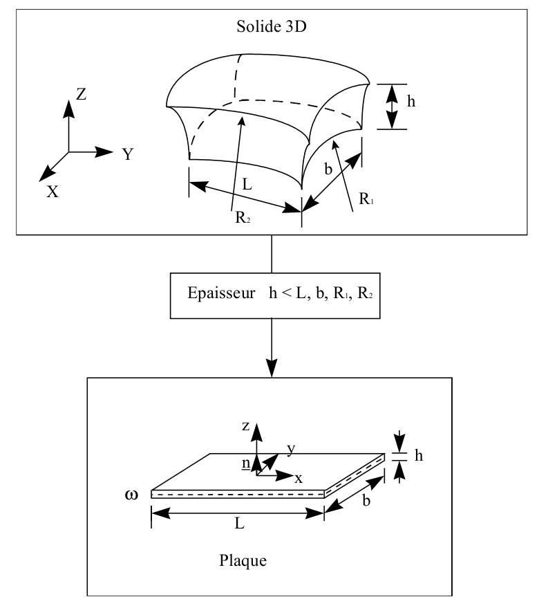
A local orthonormal coordinate system \(\mathit{Oxyz}\) associated with the tangential plane of the structure different from the global coordinate system \(\mathit{OXYZ}\) is attached to the mean surface \(\omega\). The position of the points on the plate is given by the Cartesian coordinates \((x,y)\) of the mean surface and the elevation \(z\) with respect to this surface.

2.2. Cinematics

The basic kinematics of the T3G element are Hencky-Mindlin kinematics (see [7] for details), where the 3D strain tensor, \(\varepsilon\), is defined as follows:

\({\varepsilon }_{\mathit{xx}}\mathrm{=}{e}_{\mathit{xx}}+z{\kappa }_{\mathit{xx}}\) \({\varepsilon }_{\mathit{yy}}\mathrm{=}{e}_{\mathit{yy}}+z{\kappa }_{\mathit{yy}}\) \({\varepsilon }_{\mathit{xy}}\mathrm{=}{e}_{\mathit{xy}}+z{\kappa }_{\mathit{xy}}\)

\({\varepsilon }_{\mathit{xz}}\mathrm{=}{\gamma }_{x}\) \({\varepsilon }_{\mathit{yz}}\mathrm{=}{\gamma }_{y}\) (1)

where

\({e}_{\mathit{xx}}\mathrm{=}\frac{\mathrm{\partial }u}{\mathrm{\partial }x}\) \({e}_{\mathit{yy}}\mathrm{=}\frac{\mathrm{\partial }v}{\mathrm{\partial }y}\) \({e}_{\mathit{xy}}\mathrm{=}\frac{1}{2}(\frac{\mathrm{\partial }u}{\mathrm{\partial }y}+\frac{\mathrm{\partial }v}{\mathrm{\partial }x})\)

\({\kappa }_{\mathit{xx}}=\frac{\partial {\beta }_{x}}{\partial x}\) \({\kappa }_{\mathit{yy}}\mathrm{=}\frac{\mathrm{\partial }{\beta }_{y}}{\mathrm{\partial }y}\) \({\kappa }_{\mathit{xy}}\mathrm{=}\frac{1}{2}(\frac{\mathrm{\partial }{\beta }_{x}}{\mathrm{\partial }y}+\frac{\mathrm{\partial }{\beta }_{y}}{\mathrm{\partial }x})\)

\({\beta }_{x}={\theta }_{y}\) \({\beta }_{y}\mathrm{=}\mathrm{-}{\theta }_{x}\)

\({\gamma }_{x}\mathrm{=}{\beta }_{x}+\frac{\mathrm{\partial }w}{\mathrm{\partial }x}\) \({\gamma }_{y}\mathrm{=}{\beta }_{y}+\frac{\mathrm{\partial }w}{\mathrm{\partial }y}\) (2)

\({e}_{\alpha \beta }\) being the membrane extension tensor, \({\kappa }_{\alpha \beta }\) the curvature variation tensor, \({\beta }_{x}\), \({\beta }_{y}\) the auxiliary variables defined above and \({\gamma }_{x}\), \({\gamma }_{y}\) the transverse distortions. The main variables are the movements \(u\), \(v\), \(w\) and the rotations \({\theta }_{x}\), \({\theta }_{y}\), and \({\theta }_{z}\). In the formulations considered here, the rotation normal to the mean surface, \({\theta }_{z}\), is introduced exclusively for reasons of compatibility between the nodal degrees of freedom for non-plane geometries.

2.3. Finite element support

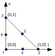
The finite element has a T3 mesh as a support, with 6 degrees of freedom per node, which makes 18 degrees of freedom in total. The main characteristics are given in the table below. We define the same shape functions for displacements, \((u,\text{}v,\text{}w)\), as for rotations, \(({\theta }_{x}\text{},\text{}{\theta }_{x})\).

TRIA3	\({N}_{i}(i\mathrm{=}\mathrm{1,}n)\)
	\(i=1à3\) \({N}^{1}(\xi ,\eta )\mathrm{=}\lambda \mathrm{=}1\mathrm{-}\xi \mathrm{-}\eta\) \({N}^{2}(\xi ,\eta )\mathrm{=}\xi\) \({N}^{3}(\xi ,\eta )=\eta\)	Three collocation points (4,5,6) to determine \({\gamma }_{x}\) and \({\gamma }_{y}\) One integration point in \((\xi \mathrm{=}\frac{1}{3};\eta \mathrm{=}\frac{1}{3})\)

Table 2.1: Finite reference element T3G used in the triangular-based Q4GG formulation

2.4. Membrane-Flexion

The present formulation is based on 5 degrees of freedom while neglecting any effect of rotation perpendicular to the middle sheet. This third rotation, represented by \({\theta }_{z}\) in the local coordinate system, is not presented in this formulation, see [7] for more details.

Membrane extension and curvature variation are discretized in an equivalent manner. The same shape functions are used for displacements and rotations, which leads to:

\({U}_{i}={N}^{r}{u}_{i}^{r}\), \({\beta }_{i}={N}^{r}{\beta }_{i}^{r}\) \((r=1à3)\)

\({u}_{i}^{r}\) and \({\beta }_{i}^{r}\) being the nodal values of the displacements and the rotations (transformed), respectively. By following equations (1) and (2) we have:

\({e}_{\mathit{ij}}\mathrm{=}{B}_{\mathit{ijk}}^{r}{u}_{k}^{r}\), \({\kappa }_{\mathit{ij}}={B}_{\mathit{ijk}}^{r}{\beta }_{k}^{r}\),

\({B}_{\mathit{ijk}}^{r}\mathrm{=}\frac{1}{2}\frac{\mathrm{\partial }{N}^{r}}{\mathrm{\partial }{\xi }_{l}}({J}_{\mathit{lj}}^{\mathrm{-}1}{\delta }_{\mathit{ik}}+{J}_{\mathit{li}}^{\mathrm{-}1}{\delta }_{\mathit{jk}})\)

Where is the Jacobian for transformation introduced on the reference element:

\({J}_{\mathit{ij}}\mathrm{=}\frac{\mathrm{\partial }{x}_{i}}{\mathrm{\partial }{\xi }_{j}}\mathrm{=}\frac{\mathrm{\partial }{N}^{r}}{\mathrm{\partial }{\xi }_{j}}{x}_{i}^{r}\)

Thus, for the functions defined in Table 2.1 and by choosing the local coordinate system of an element such as \({x}_{1}\mathrm{=}{y}_{1}\mathrm{=}{y}_{2}\mathrm{=}0\), we obtain:

\(\text{J}\mathrm{=}(\begin{array}{cc}{x}_{2}& {x}_{3}\\ 0& {y}_{3}\end{array})\); \({\text{J}}^{\mathrm{-}1}\mathrm{=}\frac{1}{{x}_{2}{y}_{3}}(\begin{array}{cc}{y}_{3}& \mathrm{-}{x}_{3}\\ 0& {x}_{2}\end{array})\)

\(\frac{\mathrm{\partial }{N}^{r}}{\mathrm{\partial }{\xi }_{k}}\mathrm{=}(\begin{array}{cc}\mathrm{-}1& \mathrm{-}1\\ 1& 0\\ 0& 1\end{array})\)

and finally the uniform membrane deformation tensor on the element:

\((\begin{array}{c}{e}_{11}\\ {e}_{22}\\ 2{e}_{12}\end{array})\mathrm{=}\frac{1}{{x}_{2}{y}_{3}}(\begin{array}{cccccc}\mathrm{-}{y}_{3}& 0& {y}_{3}& 0& 0& 0\\ 0& {x}_{3}\mathrm{-}{x}_{2}& 0& \mathrm{-}{x}_{3}& 0& {x}_{2}\\ {x}_{3}\mathrm{-}{x}_{2}& \mathrm{-}{y}_{3}& \mathrm{-}{x}_{3}& {y}_{3}& {x}_{2}& 0\end{array})(\begin{array}{c}{u}^{1}\\ {v}^{1}\\ {u}^{2}\\ {v}^{2}\\ {u}^{3}\\ {v}^{3}\end{array})\) (3)

\((\begin{array}{c}{\kappa }_{11}\\ {\kappa }_{22}\\ 2{\kappa }_{12}\end{array})\mathrm{=}\frac{1}{{x}_{2}{y}_{3}}(\begin{array}{cccccc}0& \mathrm{-}{y}_{3}& 0& {y}_{3}& 0& 0\\ \mathrm{-}({x}_{3}\mathrm{-}{x}_{2})& 0& \mathrm{-}{x}_{3}& 0& \mathrm{-}{x}_{2}& 0\\ {y}_{3}& {x}_{3}\mathrm{-}{x}_{2}& \mathrm{-}{y}_{3}& \mathrm{-}{x}_{3}& 0& {x}_{2}\end{array})(\begin{array}{c}{\theta }_{x}^{1}\\ {\theta }_{y}^{1}\\ {\theta }_{x}^{2}\\ {\theta }_{y}^{2}\\ {\theta }_{x}^{3}\\ {\theta }_{y}^{3}\end{array})\) (4)

2.5. Transverse distortion

2.5.1. Demonstration of transverse shear locking

To avoid shear locking, it is necessary to carefully choose the discretization of the transverse distortion. For example, by imposing,

\({\gamma }_{x}\mathrm{=}{\beta }_{x}+\frac{\mathrm{\partial }w}{\mathrm{\partial }x}\) and \({\gamma }_{y}\mathrm{=}{\beta }_{y}+\frac{\mathrm{\partial }w}{\mathrm{\partial }y}\) (5)

Depending on the degrees of freedom:

\((\begin{array}{c}{\gamma }_{x}\\ {\gamma }_{y}\end{array})\mathrm{=}(\begin{array}{c}{\theta }_{y}+\frac{\mathrm{\partial }w}{\mathrm{\partial }x}\\ \mathrm{-}{\theta }_{x}+\frac{\mathrm{\partial }w}{\mathrm{\partial }y}\end{array})\mathrm{=}(\begin{array}{c}{N}^{\alpha }{\theta }_{y}^{\alpha }+\frac{\mathrm{\partial }{N}^{\alpha }}{\mathrm{\partial }{\xi }_{k}}{J}_{\mathit{k1}}^{\mathrm{-}1}{w}^{\alpha }\\ \mathrm{-}{N}^{\alpha }{\theta }_{x}^{\alpha }+\frac{\mathrm{\partial }{N}^{\alpha }}{\mathrm{\partial }{\xi }_{k}}{J}_{\mathit{k2}}^{\mathrm{-}1}{w}^{\alpha }\end{array})\)

The thin plate limit, where \(h\to 0\) and therefore \({\gamma }_{x}\to 0\), \({\gamma }_{y}\to 0\) leads to the following equations at all points \((\xi ,\eta )\): \((\begin{array}{c}{\gamma }_{x}\\ {\gamma }_{y}\end{array})\mathrm{=}(\begin{array}{c}{\theta }_{y}^{1}+\frac{1}{{x}_{2}}({w}_{2}\mathrm{-}{w}_{1})+({\theta }_{y}^{2}\mathrm{-}{\theta }_{y}^{1})\xi +({\theta }_{y}^{3}\mathrm{-}{\theta }_{y}^{1})\eta \\ \mathrm{-}{\theta }_{x}^{1}+\frac{1}{{x}_{2}{y}_{3}}(({x}_{3}\mathrm{-}{x}_{2}){w}_{1}\mathrm{-}{x}_{3}{w}_{2}+{x}_{2}{w}_{3})\mathrm{-}({\theta }_{x}^{2}\mathrm{-}{\theta }_{x}^{1})\xi \mathrm{-}({\theta }_{x}^{3}\mathrm{-}{\theta }_{x}^{1})\eta \end{array})\mathrm{=}(\begin{array}{c}0\\ 0\end{array})\text{,}\mathrm{\forall }\xi ,\eta\) (6)

The conditions in equation \((6)\) lead directly to relationships \({\theta }_{x}^{3}\mathrm{=}{\theta }_{x}^{2}\mathrm{=}{\theta }_{x}^{1}\) and \({\theta }_{y}^{3}\mathrm{=}{\theta }_{y}^{2}\mathrm{=}{\theta }_{y}^{1}\). The flexural rotations are therefore all equal and necessarily zero if rigid body movements are correctly suppressed from the system. Shear locking is thus observed: a thin plate (\(h\mathrm{\approx }0\)) with the kinematics of the transverse distortion described in equation \((5)\) cannot be deformed under bending.

2.5.2. Remedy for lockdowns through the T3G approach

To remedy the locks and in a manner similar to the Q4G formulation [7], the T3G formulation uses an interpolation of the transverse distortion independent of displacements and rotations. The relationships (5) are relaxed, thanks to three collocation points. First, it is assumed that the spatial variation of the transverse distortion is linear with a constant tangential component on each edge. Second, as in Q4G, compatibility is imposed at the midpoints of the three edges and only in the tangential direction.

The values of the transverse distortion along the edges can be calculated directly as follows:

\({\gamma }_{s}^{k}\mathrm{=}\frac{{w}_{j}\mathrm{-}{w}_{i}}{{L}_{k}}+\frac{1}{2}({\beta }_{s}^{\mathit{ki}}+{\beta }_{s}^{\mathit{kj}})\) (7)

where \({\gamma }_{s}^{k}\) is the tangential component of the transverse distortion on edge \(k\), which is located between nodes \(i\) and \(j\). \({L}_{k}\) is the length of the edge \(k\) ; \({\beta }_{s}^{\mathit{ki}}\) and \({\beta }_{s}^{\mathit{kj}}\) are the projected values of the rotations (transformed) onto the tangent of the edge \(k\), corresponding to the nodes \(i\) and \(j\), respectively:

\({\beta }_{s}^{\mathit{ki}}\mathrm{=}{\beta }_{x}^{i}\mathrm{cos}{\Omega }_{k}+{\beta }_{y}^{i}\mathrm{sin}{\Omega }_{k}\)

where \({\Omega }_{k}\) represents the angle of the \(k\) edge in relation to the x-axis of the local coordinate system. Equation (7) can be rewritten as follows:

\((\begin{array}{c}{\gamma }_{s}^{1}\\ {\gamma }_{s}^{2}\\ {\gamma }_{s}^{3}\end{array})\mathrm{=}(\begin{array}{ccccccccc}\frac{1}{2}{C}_{1}& \frac{1}{2}{S}_{1}& \mathrm{-}\frac{1}{{L}_{1}}& \frac{1}{2}{C}_{1}& \frac{1}{2}{S}_{1}& \frac{1}{{L}_{1}}& 0& 0& 0\\ 0& 0& 0& \frac{1}{2}{C}_{2}& \frac{1}{2}{S}_{2}& \mathrm{-}\frac{1}{{L}_{2}}& \frac{1}{2}{C}_{2}& \frac{1}{2}{S}_{2}& \frac{1}{{L}_{2}}\\ \frac{1}{2}{C}_{3}& \frac{1}{2}{S}_{3}& \frac{1}{{L}_{3}}& 0& 0& 0& \frac{1}{2}{C}_{3}& \frac{1}{2}{S}_{3}& \mathrm{-}\frac{1}{{L}_{3}}\end{array})(\begin{array}{c}{\beta }_{x}^{1}\\ {\beta }_{y}^{1}\\ {w}_{1}\\ {\beta }_{x}^{2}\\ {\beta }_{y}^{2}\\ {w}_{2}\\ {\beta }_{x}^{3}\\ {\beta }_{y}^{3}\\ {w}_{3}\end{array})\) (8)

or \({C}_{k}\mathrm{=}\mathrm{cos}{\Omega }_{k}\) and \({S}_{k}\mathrm{=}\mathrm{sin}{\Omega }_{k}\)

On the other hand, the following form of the spatial variation is imposed in the reference frame of reference for the transverse distortion:

\(\begin{array}{c}{\gamma }_{x}\text{=}\\ {\gamma }_{y}\text{=}\end{array}\begin{array}{c}{a}_{x}+{b}_{x}\xi +{c}_{x}\eta \\ {a}_{y}+{b}_{y}\xi +{c}_{y}\eta \end{array}\) (9)

where \({a}_{x}\), \({a}_{y}\), \({b}_{x}\), \({b}_{y}\), \({c}_{x}\), \({c}_{y}\) are the parameters to be determined based on the assumptions that the tangential components of \(\gamma\) are constant on each edge.

So we get:

math:

{gamma} _ {s} ^ {1}mathrm {=} {gamma} _ {x} {text {|}} _ {etamathrm {=} 0}mathrm {=} 0}}mathrm {=} ^ {1}}{1}1}mathrm {=} {1}{1}mathrm {=} {0}}}mathrm {=} {0}}mathrm {=} {0}}mathrm {=} {0}}mathrm {=} {0}}mathrm {=} {0}}mathrm {=} {0}}mathrm {=} {0}}mathrm {=} {gamma} _ {s} ^ {1}text {},text {} {b} _ {x} =0

math:

{gamma} _ {s} ^ {2}mathrm {=} ({gamma} _ {x} {C} _ {2} + {gamma} _ {y} {S} _ {2} _ {2}) {text {|}}) {text {|}}) {text {|}}) {text {|}}) {text {|}}} _ {eta +ximathrm {=} 1}mathrm {=}}mathrm {=} _ {2}) {text {|} {2}) {text {|}}) {text {|}}) {text {|}}} _ {eta +ximathrm {=} 1}mathrm {} _ {x} {C} _ {2} + {a} + {a} _ {y} {S} _ {2} + {c} _ {x} {C} _ {2} + ({b} _ {y} {S}} {S} _ {2} _ {2}mathrm {-} {S} _ {y} {S} _ {y} {S} _ {y} {S} _ {y} {S} _ {y} {S} _ {y} {S} _ {y} {S} _ {y} {S} _ {y} {S} _ {y} {S} _ {y} {S} _ {y} {S} _ {y} {S} _ {y} {S} _ {y} {S} _ {y} {S} _ {2})ximathrm {]}

\(\to \text{}{a}_{x}{C}_{2}+{a}_{y}{S}_{2}+{c}_{x}{C}_{2}={\gamma }_{s}^{2}\text{}\text{;}\) \({b}_{y}{S}_{2}\mathrm{-}{c}_{x}{C}_{2}\mathrm{-}{c}_{y}{S}_{2}\mathrm{=}0\)

\({\gamma }_{s}^{3}\mathrm{=}{({\gamma }_{x}{C}_{3}+{\gamma }_{y}{S}_{3})}_{\xi \mathrm{=}0}\mathrm{=}{a}_{x}{C}_{3}+{a}_{y}{S}_{3}+({c}_{x}{C}_{3}+{c}_{y}{S}_{3})\eta\)

\(\to \text{}{a}_{x}{C}_{3}+{a}_{y}{S}_{3}={\gamma }_{s}^{3}\text{}\text{;}\) \({c}_{x}{C}_{3}+{c}_{y}{S}_{3}=0\)

What leads to the end result

\({a}_{x}\mathrm{=}{\gamma }_{s}^{1}\), \({a}_{y}\mathrm{=}\mathrm{-}\frac{{C}_{3}}{{S}_{3}}{\gamma }_{s}^{1}+\frac{1}{{S}_{3}}{\gamma }_{s}^{3}\)

\({b}_{x}\mathrm{=}0\), \({b}_{y}\mathrm{=}\mathrm{-}\frac{1}{{\mathit{QS}}_{2}}{\gamma }_{s}^{1}+\frac{1}{{S}_{2}}{\gamma }_{s}^{2}\mathrm{-}\frac{1}{{S}_{3}}{\gamma }_{s}^{3}\)

\({c}_{x}\mathrm{=}\mathrm{-}{\gamma }_{s}^{1}+Q{\gamma }_{s}^{2}\mathrm{-}Q\frac{{S}_{2}}{{S}_{3}}{\gamma }_{s}^{3}\), \({c}_{y}\mathrm{=}\frac{{C}_{3}}{{S}_{3}}{\gamma }_{s}^{1}\mathrm{-}Q\frac{{C}_{3}}{{S}_{3}}{\gamma }_{s}^{2}+Q\frac{{C}_{3}{S}_{2}}{{S}_{3}^{2}}{\gamma }_{s}^{3}\) (10)

Where \(Q=1/({C}_{2}-{S}_{2}\frac{{C}_{3}}{{S}_{3}})\)

From equations \((9)\) and \((10)\) we can write:

\((\begin{array}{c}{\gamma }_{x}\\ {\gamma }_{y}\end{array})\mathrm{=}(\begin{array}{ccc}1\mathrm{-}\eta & Q\eta & \mathrm{-}\frac{{S}_{2}}{{S}_{3}}Q\eta \\ \mathrm{-}\frac{{C}_{3}}{{S}_{3}}\mathrm{-}\frac{1}{{\mathit{QS}}_{2}}\xi +\frac{{C}_{3}}{{S}_{3}}\eta & \frac{1}{{S}_{2}}\xi \mathrm{-}\frac{{C}_{3}}{{S}_{3}}Q\eta & \frac{1}{{S}_{3}}\mathrm{-}\frac{1}{{S}_{3}}\xi +\frac{{C}_{3}{S}_{2}}{{S}_{3}^{2}}Q\eta \end{array})(\begin{array}{c}{\gamma }_{s}^{1}\\ {\gamma }_{s}^{2}\\ {\gamma }_{s}^{3}\end{array})\) (11)

By combining equations \((8)\) and \((11)\) we get:

\((\begin{array}{c}{\gamma }_{x}\\ {\gamma }_{y}\end{array})\mathrm{=}(\begin{array}{ccc}1\mathrm{-}\eta & Q\eta & \mathrm{-}\frac{{S}_{2}}{{S}_{3}}Q\eta \\ \mathrm{-}\frac{{C}_{3}}{{S}_{3}}\mathrm{-}\frac{1}{{\mathit{QS}}_{2}}\xi +\frac{{C}_{3}}{{S}_{3}}\eta & \frac{1}{{S}_{2}}\xi \mathrm{-}\frac{{C}_{3}}{{S}_{3}}Q\eta & \frac{1}{{S}_{3}}\mathrm{-}\frac{1}{{S}_{3}}\xi +\frac{{C}_{3}{S}_{2}}{{S}_{3}^{2}}Q\eta \end{array})\mathrm{\times }\text{}\)

\((\begin{array}{ccccccccc}\frac{1}{2}& 0& \mathrm{-}\frac{1}{{L}_{1}}& \frac{1}{2}& 0& \frac{1}{{L}_{1}}& 0& 0& 0\\ 0& 0& 0& \frac{1}{2}{C}_{2}& \frac{1}{2}{S}_{2}& \mathrm{-}\frac{1}{{L}_{2}}& \frac{1}{2}{C}_{2}& \frac{1}{2}{S}_{2}& \frac{1}{{L}_{2}}\\ \frac{1}{2}{C}_{3}& \frac{1}{2}{S}_{3}& \frac{1}{{L}_{3}}& 0& 0& 0& \frac{1}{2}{C}_{3}& \frac{1}{2}{S}_{3}& \mathrm{-}\frac{1}{{L}_{3}}\end{array})(\begin{array}{c}{\beta }_{x}^{1}\\ {\beta }_{y}^{1}\\ {w}_{1}\\ {\beta }_{x}^{2}\\ {\beta }_{y}^{2}\\ {w}_{2}\\ {\beta }_{x}^{3}\\ {\beta }_{y}^{3}\\ {w}_{3}\end{array})\) (12)

The expressions above have been slightly simplified by using the same local coordinate system as in [§2.4], i.e. the one where \({\Omega }_{1}\mathrm{=}0\) and therefore \({C}_{1}\mathrm{=}1\) and \({S}_{1}\mathrm{=}0\). The relationship between the degrees of freedom of the element, \({U}_{i}^{\alpha }\) and the transverse distortion at any point \((\xi ,\eta )\), of equation \((12)\) is written in the form:

\({\gamma }_{i}\mathrm{=}{B}_{\mathit{ik}\alpha }^{\mathit{ct}}(\xi ,\eta ){U}_{k}^{\alpha }\)

Where

\({\text{B}}^{\mathit{ct}}\mathrm{=}(\begin{array}{ccc}1\mathrm{-}\eta & Q\eta & \mathrm{-}\frac{{S}_{2}}{{S}_{3}}Q\eta \\ \mathrm{-}\frac{{C}_{3}}{{S}_{3}}\mathrm{-}\frac{1}{{\mathit{QS}}_{2}}\xi +\frac{{C}_{3}}{{S}_{3}}\eta & \frac{1}{{S}_{2}}\xi \mathrm{-}\frac{{C}_{3}}{{S}_{3}}Q\eta & \frac{1}{{S}_{3}}\mathrm{-}\frac{1}{{S}_{3}}\xi +\frac{{C}_{3}{S}_{2}}{{S}_{3}^{2}}Q\eta \end{array})\mathrm{\times }\text{}\)

\((\begin{array}{ccccccccc}\frac{1}{2}& 0& \mathrm{-}\frac{1}{{L}_{1}}& \frac{1}{2}& 0& \frac{1}{{L}_{1}}& 0& 0& 0\\ 0& 0& 0& \frac{1}{2}{C}_{2}& \frac{1}{2}{S}_{2}& \mathrm{-}\frac{1}{{L}_{2}}& \frac{1}{2}{C}_{2}& \frac{1}{2}{S}_{2}& \frac{1}{{L}_{2}}\\ \frac{1}{2}{C}_{3}& \frac{1}{2}{S}_{3}& \frac{1}{{L}_{3}}& 0& 0& 0& \frac{1}{2}{C}_{3}& \frac{1}{2}{S}_{3}& \mathrm{-}\frac{1}{{L}_{3}}\end{array})\)

and

\(U\mathrm{=}{(\begin{array}{ccccccccc}{\beta }_{x}^{1}& {\beta }_{y}^{1}& {w}_{1}& {\beta }_{x}^{2}& {\beta }_{y}^{2}& {w}_{2}& {\beta }_{x}^{3}& {\beta }_{y}^{3}& {w}_{3}\end{array})}^{T}\)

Contrary to the discretization explained in [§2.5.1], and in equation \((5)\), the limit \(h\to 0\) applied to independent kinematics leads to three equations that couple in a more balanced way the displacements \(w\), and the rotations \({\theta }_{x}\), \({\theta }_{y}\), and the rotations,, according to the equation \((8)\).

\((\begin{array}{c}0\\ 0\\ 0\end{array})\mathrm{=}(\begin{array}{ccccccccc}\frac{1}{2}{C}_{1}& \frac{1}{2}{S}_{1}& \mathrm{-}\frac{1}{{L}_{1}}& \frac{1}{2}{C}_{1}& \frac{1}{2}{C}_{2}& \frac{1}{{L}_{1}}& 0& 0& 0\\ 0& 0& 0& \frac{1}{2}{C}_{2}& \frac{1}{2}{S}_{2}& \mathrm{-}\frac{1}{{L}_{2}}& \frac{1}{2}{C}_{2}& \frac{1}{2}{S}_{2}& \frac{1}{{L}_{2}}\\ \frac{1}{2}{C}_{3}& \frac{1}{{S}_{3}}& \frac{1}{{L}_{3}}& 0& 0& 0& \frac{1}{2}{C}_{3}& \frac{1}{2}{S}_{3}& \mathrm{-}\frac{1}{{L}_{3}}\end{array})(\begin{array}{c}{\beta }_{x}^{1}\\ {\beta }_{y}^{1}\\ {w}_{1}\\ {\beta }_{x}^{2}\\ {\beta }_{y}^{2}\\ {w}_{2}\\ {\beta }_{x}^{3}\\ {\beta }_{y}^{3}\\ {w}_{3}\end{array})\) (13)

The conditions in equation \((13)\) do not cause any blockage on the rotational degrees of freedom. Moreover, in equation \((13)\) we used equation \((11)\) to deduce that

\((\begin{array}{c}{\gamma }_{x}\\ {\gamma }_{y}\end{array})\mathrm{=}(\begin{array}{c}0\\ 0\end{array})\)

at all points, only if:

\((\begin{array}{c}{\gamma }_{s}^{1}\\ {\gamma }_{s}^{2}\\ {\gamma }_{s}^{3}\end{array})\mathrm{=}(\begin{array}{c}0\\ 0\\ 0\end{array})\)

2.6. Calculation of stresses and internal forces

The application of the kinematics defined in [§2.4] to the calculation of internal forces is presented here. Two different cases will be considered:

• Linear elasticity,

• Global model type GLRC.

For linear elasticity, only one integration point in the thickness is required, as deformations and stresses vary linearly in the thickness.

The main objective of Q4GG modeling is the use of the GLRC_DAMAGE [R7.01.31] model as part of the T3G and Q4G element. A single integration point in the thickness is necessary, as non-linearity is taken into account directly in terms of generalized forces and deformations.

2.6.1. Linear elasticity

For linear elastic behavior, potential energy is defined as follows:

\({\Phi }^{L}\mathrm{=}\frac{1}{2}{\mathrm{\int }}_{S}{\mathrm{\int }}_{\frac{\mathrm{-}h}{2}}^{\text{}\frac{h}{2}}{\varepsilon }_{\mathit{ij}}{C}_{\mathit{ijkl}}^{\mathit{el}}{\varepsilon }_{\mathit{kl}}\mathit{dz}\mathit{dS}+{\Phi }^{\mathit{ext}}\)

\(\text{}\mathrm{=}\frac{1}{2}{\mathrm{\int }}_{S}\mathrm{[}{e}_{\mathit{ij}}{H}_{\mathit{ijkl}}^{M}{e}_{\mathit{kl}}+{\kappa }_{\mathit{ij}}{H}_{\mathit{ijkl}}^{M}{\kappa }_{\mathit{kl}}+{\gamma }_{i}{H}_{\mathit{ij}}^{\mathit{CT}}{\gamma }_{j}\mathrm{]}\mathit{dS}+{\Phi }^{\mathit{ext}}\) (14)

where \(\epsilon\) and \({\text{C}}^{\mathit{el}}\) are, respectively, the deformation tensor \(\mathrm{3D}\) and the corresponding elastic tensor. For a linear material, the integral according to \(z\) takes place analytically. \({\Phi }^{\mathit{ext}}\) represents the contribution due to the boundary conditions. The tensors \(e\), \(\kappa\), represent membrane extension and curvature variation and the vector \(\gamma\) represents transverse distortion, as introduced in [§2.4]. In equation \((14)\), it is also assumed that the shell is symmetric with respect to the middle sheet, otherwise an additional membrane-flexure coupling term is obtained. The calculation details in equation \((14)\) are provided in [7], where we find the following expressions for the \(\text{H}\) matrices:

\({\text{H}}^{M}=\frac{\mathit{Eh}}{1-{\nu }^{2}}\left(\begin{array}{ccc}1& \nu & 0\\ \nu & 1& 0\\ 0& 0& \frac{1-\nu }{2}\end{array}\right)\) \({\text{H}}^{F}=\frac{{\mathit{Eh}}^{3}}{12(1-{\nu }^{2})}\left(\begin{array}{ccc}1& \nu & 0\\ \nu & 1& 0\\ 0& 0& \frac{1-\nu }{2}\end{array}\right)\) \({\text{H}}^{\mathit{CT}}=\frac{\mathit{kEh}}{2(1+\nu )}\left(\begin{array}{cc}1& 0\\ 0& 1\end{array}\right)\)

where \(h\) is the thickness, \(E\) is the Young’s modulus, \(\nu\) is the Poisson’s ratio, and \(k\) is a parameter that can vary depending on the theory applied. Most often \(k=\frac{5}{6}\) (Reissner model) is used.

Then, we apply the kinematics introduced in [§2.3] and [§2.4]:

\(\left(\begin{array}{c}{e}_{\mathit{xx}}\\ {e}_{\mathit{yy}}\\ {e}_{\mathit{xy}}\end{array}\right)={\text{B}}^{M}\left(\begin{array}{c}{u}^{1}\\ {v}^{1}\\ {u}^{2}\\ {v}^{2}\\ {u}^{3}\\ {v}^{3}\end{array}\right)\) \(\left(\begin{array}{c}{\kappa }_{\mathit{xx}}\\ {\kappa }_{\mathit{yy}}\\ {\kappa }_{\mathit{xy}}\end{array}\right)={\text{B}}^{F}\left(\begin{array}{c}{\theta }_{x}^{1}\\ {\theta }_{y}^{1}\\ {\theta }_{x}^{2}\\ {\theta }_{y}^{2}\\ {\theta }_{x}^{3}\\ {\theta }_{y}^{3}\end{array}\right)\) \(\left(\begin{array}{c}{\gamma }_{x}\\ {\gamma }_{y}\end{array}\right)={\text{B}}^{\mathit{CT}}\left(\begin{array}{c}{\theta }_{x}^{1}\\ {\theta }_{y}^{1}\\ {w}^{1}\\ {\theta }_{x}^{2}\\ {\theta }_{y}^{2}\\ {w}^{2}\\ {\theta }_{x}^{3}\\ {\theta }_{y}^{3}\\ {w}^{3}\end{array}\right)\)

to get from equation \((14)\):

\({\Phi }^{L}\mathrm{=}\frac{1}{2}{U}_{\alpha }^{T}\underset{{K}_{\alpha \beta }^{M}}{\underset{\underbrace{}}{\mathrm{[}{\mathrm{\int }}_{S}{B}_{\mathit{ij}\alpha }^{M}{H}_{\mathit{ijkl}}^{M}{B}_{\mathit{kl}\beta }^{M}\mathit{dS}\mathrm{]}}}{U}_{\beta }+\frac{1}{2}{U}_{\alpha }^{T}\underset{{K}_{\alpha \beta }^{F}}{\underset{\underbrace{}}{\mathrm{[}{\mathrm{\int }}_{S}{B}_{\mathit{ij}\alpha }^{F}{H}_{\mathit{ijkl}}^{F}{B}_{\mathit{kl}\beta }^{F}\mathit{dS}\mathrm{]}}}{U}_{\beta }+\text{}\)

\(\frac{1}{2}{U}_{\alpha }^{T}\underset{{K}_{\alpha \beta }^{\mathit{CT}}}{\underset{\underbrace{}}{\mathrm{[}{\mathrm{\int }}_{S}{B}_{\mathit{ij}\alpha }^{\mathit{CT}}{H}_{\mathit{ijkl}}^{\mathit{CT}}{B}_{\mathit{kl}\beta }^{\mathit{CT}}\mathit{dS}\mathrm{]}}}{U}_{\beta }+{\Phi }^{\mathit{ext}}\)

By using the principle of minimum free energy, \(\mathrm{\partial }{\Phi }^{L}\mathrm{=}0\), \(\mathrm{\forall }\delta {U}_{\alpha }\), we obtain:

\(\underset{{\text{F}}^{\text{int}}}{\underset{\underbrace{}}{({K}_{\alpha \beta }^{M}+{K}_{\alpha \beta }^{F}+{K}_{\alpha \beta }^{\mathit{CT}}){U}_{\beta }}}\mathrm{=}{F}_{\alpha }^{\mathit{ext}}\)

where \({\text{F}}^{\text{int}}\) and \({\text{F}}^{\text{ext}}\) are, respectively, the internal and external forces.

The integration of all the contributions to the stiffness matrix \({\text{K}}^{M}\), \({\text{K}}^{F}\), and \({\text{K}}^{\mathit{CT}}\) takes place with a single integration point in the triangle plane (center of gravity). This gives an exact integration for the terms \({\text{K}}^{M}\) and \({\text{K}}^{F}\) because \({\text{H}}^{M}\), \({\text{H}}^{F}\), \({\text{B}}^{M}\), \({\text{B}}^{F}\) are element-wise constants (see [§4.5]). In contrast, \({\text{B}}^{\mathit{CT}}\) is a linear function (see [§2.4]) and the exact integration of \({\text{K}}^{\mathit{CT}}\) would require three Gauss points.

As the T3G element, as proposed in [3] and discussed in [12], is under-integrated on the transverse shear portion, it has a parasitic mode, i.e. a zero energy mode, which is not a rigid body mode. However, based on two elements, the T3G model regains a correct « rank ».

2.6.2. Global non-linear behavior of type GLRC

When using a global model, the relationship between stresses and strains is defined in terms of generalized variables, \({\varepsilon }^{G}\), \({\sigma }^{G}\):

\({\varepsilon }^{G}\mathrm{=}(\begin{array}{c}e\\ \kappa \\ \gamma \end{array})\) \({\sigma }^{G}\mathrm{=}(\begin{array}{c}N\\ M\\ T\end{array})\)

where the generalized deformations are membrane extension \(e\), curvature variation \(\kappa\), and transverse distortion \(\gamma\) (see [§2.4] for more precise definitions). The generalized stresses are membrane force \(\text{N}\), bending moment \(\text{M}\), and transverse shear \(\text{T}\):

\(\text{N}\mathrm{=}(\begin{array}{c}{N}_{\mathit{xx}}\\ {N}_{\mathit{yy}}\\ {N}_{\mathit{xy}}\end{array})\mathrm{=}\frac{1}{2}{\mathrm{\int }}_{\mathrm{-}\frac{h}{2}}^{\text{}\frac{h}{2}}(\begin{array}{c}{\sigma }_{\mathit{xx}}\\ {\sigma }_{\mathit{yy}}\\ {\sigma }_{\mathit{xy}}\end{array})\mathit{dz}\) \(\text{M}\mathrm{=}(\begin{array}{c}{M}_{\mathit{xx}}\\ {M}_{\mathit{yy}}\\ {M}_{\mathit{xy}}\end{array})\mathrm{=}\frac{1}{2}{\mathrm{\int }}_{\mathrm{-}\frac{h}{2}}^{\text{}\frac{h}{2}}z(\begin{array}{c}{\sigma }_{\mathit{xx}}\\ {\sigma }_{\mathit{yy}}\\ {\sigma }_{\mathit{xy}}\end{array})\mathit{dz}\)

\(\text{T}\mathrm{=}(\begin{array}{c}{T}_{x}\\ {T}_{y}\end{array})\mathrm{=}{\mathrm{\int }}_{\mathrm{-}\frac{h}{2}}^{\text{}\frac{h}{2}}(\begin{array}{c}{\sigma }_{\mathit{xz}}\\ {\sigma }_{\mathit{yz}}\end{array})\mathit{dz}\)

Model GLRC_DAMAGE takes into account elasto-plasticity in membrane-flexure, mainly due to steels, and flexural damage, mainly due to concrete. The free energy corresponding to the model is defined as:

\({\Phi }^{G}\mathrm{=}\frac{1}{2}{\mathrm{\int }}_{S}{(e\mathrm{-}{e}^{P})}_{\mathit{ij}}{H}_{\mathit{ijkl}}^{M}{(e\mathrm{-}{e}^{p})}_{\mathit{kl}}\mathit{dS}+\frac{1}{2}{\mathrm{\int }}_{S}{(\kappa \mathrm{-}{\kappa }^{P})}_{\mathit{ij}}{H}_{\mathit{ijkl}}^{\mathit{Fd}}({d}_{\mathrm{1,}}{d}_{2}){(\kappa \mathrm{-}{\kappa }^{p})}_{\mathit{kl}}\mathit{dS}\) (15)

\(+\frac{1}{2}{\mathrm{\int }}_{S}{\gamma }_{\mathit{ij}}{H}_{\mathit{ijkl}}^{\mathit{CT}}{\gamma }_{\mathit{kl}}\mathit{dS}\)

where \({e}^{p}\) and \({\kappa }^{p}\) are, respectively, the plastic membrane extension and the plastic curvature variation; \({\text{H}}^{M}\) and \({\text{H}}^{\mathit{CT}}\) are the elastic matrices for membrane and transverse shear, the same as those defined in [§2.6.1]. For the flexure part, we define the matrix \({\text{H}}^{\mathit{Fd}}\), which is a function of the damage variables \({d}_{1}\) and \({d}_{2}\) [8]. It is noted that no non-linearity is considered for the portion of the transverse shear. This hypothesis is not really justified, because damage to concrete necessarily induces a reduction in transverse shear stiffness. Since the model was designed under the thin plate hypothesis, it is not recommended to use model GLRC_DAMAGE in situations where transverse shear energy becomes comparable to membrane or flexural contributions.

By imposing \(\mathrm{\partial }{\Phi }^{G}\mathrm{=}0\), we get:

\(\delta {\Phi }^{G}\mathrm{=}\delta {U}^{\alpha }\underset{{\text{F}}_{\text{int}}^{M}}{\underset{\underbrace{}}{{\mathrm{\int }}_{S}{({\stackrel{ˆ}{B}}_{\alpha }^{M})}^{T}(\begin{array}{c}{N}_{\mathit{xx}}\\ {N}_{\mathit{yy}}\\ {N}_{\mathit{xy}}\end{array})\mathit{dS}}}+\delta {\theta }^{\alpha }\underset{{\text{F}}_{\text{int}}^{F}}{\underset{\underbrace{}}{{\mathrm{\int }}_{S}{({\stackrel{ˆ}{B}}_{\alpha }^{F})}^{T}(\begin{array}{c}{M}_{\mathit{xx}}\\ {M}_{\mathit{yy}}\\ {M}_{\mathit{xy}}\end{array})+{({\stackrel{ˆ}{B}}_{\theta \alpha }^{\mathit{CT}})}^{T}{\text{H}}^{\mathit{CT}}(\begin{array}{c}{\gamma }_{x}\\ {\gamma }_{y}\end{array})\mathit{dS}}}\text{}\) (16)

\(+\delta {w}^{\alpha }\underset{{\text{F}}_{\text{int}}^{\mathit{CT}}}{\underset{\underbrace{}}{{\mathrm{\int }}_{s}{({\stackrel{ˆ}{B}}_{w\alpha }^{\mathit{CT}})}^{T}{\text{H}}^{\mathit{CT}}(\begin{array}{c}{\gamma }_{x}\\ {\gamma }_{y}\end{array})\mathit{dS}}}\)

where the following relationships are used:

\({\stackrel{ˆ}{\text{B}}}^{M}\mathrm{=}{\mathrm{\int }}_{\mathrm{-}\frac{h}{2}}^{\text{}\frac{h}{2}}{\text{B}}^{M}\mathit{dz}\) \({\stackrel{ˆ}{\text{B}}}^{F}\mathrm{=}{\mathrm{\int }}_{\mathrm{-}\frac{h}{2}}^{\text{}\frac{h}{2}}z{\text{B}}^{F}\mathit{dz}\) \({\stackrel{ˆ}{\text{B}}}^{\mathit{CT}}\mathrm{=}{\mathrm{\int }}_{\mathrm{-}\frac{h}{2}}^{\text{}\frac{h}{2}}{\text{B}}^{\mathit{CT}}\mathit{dz}\)

The law of behavior, almost all of whose characteristics derive from the definition of free energy [éq .4.7.3-1], can be summarized, following equation \((16)\), in terms of relationships:

\(\text{N}\mathrm{=}\text{N}(e,\kappa )\) \(\text{M}\mathrm{=}\text{M}(e,\kappa )\) \(\text{T}\mathrm{=}{\text{H}}^{\mathit{CT}}\gamma\)

Details of the application of the GLRC_DAMAGE model in a « finite element » framework are given in [4] and [8].

2.7. « Lumped » mass matrix

In this paragraph we present the approach used to build the « lumped » mass matrix. We focus on the terms due to flexure, the terms corresponding to the membrane being obtained in a conventional manner also applied to elements \(\mathrm{2D}\). The mass matrix \(\text{M}\) is defined using kinetic energy \({E}^{\mathit{cin}}\) and the kinematics proposed in [§2.2]:

\({E}^{\mathit{cin}}\mathrm{=}\frac{1}{2}{\mathrm{\int }}_{S}{\mathrm{\int }}_{\mathrm{-}\frac{h}{2}}^{\text{}\frac{h}{2}}\rho {\dot{u}}^{2}\mathit{dz}\mathit{dS}\mathrm{=}({\dot{\theta }}_{x}^{\alpha }\text{}{\dot{\theta }}_{y}^{\alpha }\text{}{\dot{w}}^{\alpha }){M}^{\alpha \beta }(\begin{array}{c}{\dot{\theta }}_{x}^{\beta }\\ {\dot{\theta }}_{y}^{\beta }\\ {\dot{w}}^{\beta }\end{array})+{E}_{\mathit{memb}}^{\mathit{cin}}\)

where \({E}_{\mathit{memb}}^{\mathit{cin}}\) represents the contribution of the membrane, \(\rho\) being the density and the mass matrix \(\text{M}\) being equal to:

\({M}^{\alpha \beta }\mathrm{=}{m}^{\alpha \beta }(\begin{array}{ccc}\frac{{h}^{3}}{12}& 0& 0\\ 0& \frac{{h}^{3}}{12}& 0\\ 0& 0& h\end{array})\) (17)

\({m}^{\alpha \beta }\mathrm{=}{\mathrm{\int }}_{s}\rho {N}^{\alpha }{N}^{\beta }\mathit{dS}\) (18)

One way to calculate the integral \((18)\) is through Gauss quadrature, which leads to the coherent matrix coupling the contributions of the different degrees of freedom. It is generally recognized that the calculation of a coherent mass matrix is not justified for calculations in fast dynamics, for which the « lumped » matrix always offers a better precision-cost ratio.

The same mass matrix is used for T3G as for DKT. In addition to the approximation of the decoupling of the different degrees of freedom, leading to the use of the lumped matrix, approximations are made on the inertia terms in order to increase the stability time step.

In [5] it is proposed to build the lumped matrix from equation \((18)\) using the Lobatto quadrature, whose variants are the trapezoidal diagram and the Simpson diagram, where the integration points coincide with the nodes. The construction of the mass matrix is carried out through a finite, linear and two-node beam element, using the trapezoidal diagram, leading to:

\({M}_{0}^{\mathit{pout}}\mathrm{=}\frac{1}{2}\rho \mathit{LA}(\begin{array}{cccc}\frac{I}{A}& 0& 0& 0\\ 0& 1& 0& 0\\ 0& 0& \frac{I}{A}& 0\\ 0& 0& 0& 1\end{array})\) (19)

for which the degrees of freedom vector is written as \({({\theta }_{1}{w}_{1}{\theta }_{2}{w}_{2})}^{T}\). \(A\), \(L\), and \(I\) are the cross-sectional area, length, and moment of inertia of the beam element, respectively. Since the use of the \((\mathit{eq.}19)\) matrix seems too restrictive compared to the condition of stability of the explicit integration scheme in time, we propose in [5] instead:

\({M}_{0}^{\mathit{pout}}\mathrm{=}\frac{1}{2}\rho \mathit{LA}(\begin{array}{cccc}\alpha & 0& 0& 0\\ 0& 1& 0& 0\\ 0& 0& \alpha & 0\\ 0& 0& 0& 1\end{array})\)

where the \(\alpha\) parameter is introduced so that its adjustment can maximize the stability time step. According to [5] its optimal value would be \(\alpha \mathrm{=}\frac{1}{8}{L}^{2}\). By directly applying these results by analogy to the plates, the matrix in equation \((19)\) is replaced by:

\({M}^{\alpha \beta }\mathrm{=}{m}^{\alpha \beta }(\begin{array}{ccc}\frac{{\mathit{hA}}^{e}}{8}& 0& 0\\ 0& \frac{{\mathit{hA}}^{e}}{8}& 0\\ 0& 0& h\end{array})\) (20)

where \({A}^{e}\) is the area of the element under consideration. In the transition from the beam to the plate a certain equivalence between the length of the beam element and the area of the plate element was assumed, so that \({A}^{e}\mathrm{\approx }{L}^{2}\). We recall that the approach proposed in [5] is not rigorous from a geometric point of view and that it focuses on maximizing the stability step. In the version implemented in Code_Aster we ensure the desired effect of modifying \((18)\) to \((19)\) by using (as was done for the elements of the DKT [7] family):

\({M}^{\alpha \beta }\mathrm{=}{m}^{\alpha \beta }(\begin{array}{ccc}\mathit{max}(\frac{{h}^{3}}{12}\text{},\text{}\frac{{\mathit{hA}}^{e}}{8})& 0& 0\\ 0& \mathit{max}(\frac{{h}^{3}}{12}\text{},\text{}\frac{{\mathit{hA}}^{e}}{8})& 0\\ 0& 0& h\end{array})\) (21)

because equation \((20)\) is only interesting for coarse meshes, which are apparently more common, while equation \((17)\) becomes favorable for very fine meshes. Moreover, in Code_Aster we decide to integrate \((18)\) by squaring Gauss at three points while keeping only the diagonal terms:

\({m}^{\alpha \beta }\mathrm{=}{\delta }_{\alpha \beta }{\mathrm{\int }}_{s}\rho {N}^{\alpha }{N}^{\beta }\mathit{dS}\) (22)

Note: the classical coherent mass matrix was not developed for this finite element in*Code_Aster*.

2.8. Second member corresponding to external work

The variational formulation of outside work and the discretization of the potential of external efforts are presented in §4.8 of [R3.07.03].

Note: Thermal loading is not treated.