2.1. Description of geometry, kinematics
We consider a shell with \(\mathit{Oy}\) axis revolution. For this shell, the mean surface is defined by the curve \(\omega \mathrm{=}\text{AB}\) in the \(O\text{xz}\) plane: \(\omega\) is a meridian for the shell of revolution.
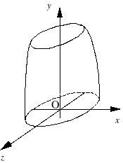
Figure 2.1-1: Revolution shell
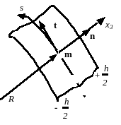
Curve \(\omega \mathrm{=}\text{AB}\) is parameterized by the curvilinear abscissa \(s\). We will denote the partial derivatives \(\frac{\partial A}{\partial s}\) of a quantity \(A\) by \({A}_{,s}\). At a point \(m\) of \(\omega\) we define the local coordinate system \((n,t,{e}_{z})\) by:
(2.1)\[ t\ mathrm {=}\ frac {{\ text {Om}}} _ {, s}} {\ mathrm {\ parallel} {\ text {Om}} _ {, s}\ mathrm {\ parallel}}\]
We also note angle \(\alpha\) such as:
(2.2)\[ n=\ text {cos}\ alpha {e} _ {x} +\ text {sin}\ alpha {e} _ {y}\]
The curvature of \(\omega\) is defined by:
(2.3)\[ \ frac {1} {R} =-n\ cdot {t} _ {, s} = {\ alpha} _ {, s}\]
The position on the parallel passing through \(m\) is noted \(\theta\). The tangent vector on this parallel is \({e}_{\theta }\). For the meridian located in plane \(\mathit{Oxz}\), \(\theta =0\), and \({e}_{\theta }=-{e}_{z}\). The radius of curvature of the parallel in \(m\) is:
\[\]
: label: eq-4
{R} _ {theta} =frac {r} {text {cos}alpha}
Where \(r\) is the \(x\) abscissa of the point \(m\) of \(\omega\). The kinematic transformations of the shell are defined by the displacement \(U\) from point \(m\) of the mean surface, as well as by the rotation \({\beta }_{s}\) from normal \(n\) to point \(m\). The vector \(U\) can be expressed in a local base:
\[\]
: label: eq-5
{U} _ {(s)} = {U} _ {(s)}cdot {t} _ {(s)} + {W} _ {(s)}cdot {n} _ {n} _ {(s)}
Or on a Cartesian basis:
(2.4)\[ {U} _ {(s)} = {u} _ {x} (s)\ cdot {e} _ {x} + {u} _ {y} (s)\ cdot {e} _ {y}\]
The deformations of the shell associated with this transformation \((U\text{,}{\beta }_{s})\) are determined by:
a membrane deformation tensor \(E\),
a \(K\) curvature variation tensor,
a \(\gamma\) transverse distortion deformation vector.
The latter appears in the shell theory of HENCKY - MINDLIN - NAGHDI and not in that of LOVE. As a function of the displacement \(U\) and the rotation \({\beta }_{s}\), these quantities are expressed (cf. [bib 1]) in the case where \(U\) is expressed in the local base \((n,t,{e}_{z})\):
(2.5)\[ {E} _ {\ mathit {ss}} = {U} _ {, s} +\ frac {W} {R}
{E} _ {\ theta\ theta} =\ frac {1} {r} (-U\ mathrm {sin}\ alpha +W\ mathrm {cos}\ alpha)
{K} _ {\ mathit {ss}} = {\ beta} _ {s, s}
{K} _ {\ theta\ theta} =-\ frac {\ text {sin}\ alpha} {r} {\ beta} _ {s}
{\ gamma} _ {s} = {\ beta} _ {s} _ {s} + {W} _ {, s} -\ frac {U} {R}\]
And for the case where \(U\) is expressed in global basis \(({e}_{x}\text{,}{e}_{y}\text{,}{e}_{z})\):
(2.6)\[ {E} _ {\ mathit {ss}} = {u} _ {y, s}\ mathrm {cos}\ alpha - {u} _ {x, s}\ mathrm {sin}\ alpha
{E} _ {\ theta\ theta} =\ frac {{u} _ {x}} {r}
{K} _ {\ mathit {ss}} = {\ beta} _ {s, s}
{K} _ {\ theta\ theta} =-\ frac {\ text {sin}\ alpha} {r} {\ beta} _ {s}
{\ gamma} _ {s} = {\ beta} _ {s} _ {s} + {u} _ {x, s}\ mathrm {cos}\ alpha + {u} _ {y, s}\ mathrm {sin}\ alpha\]
Note:
The change in the direction of the curvilinear abscissa \(s\) does not change the values of: \({\beta }_{s}\) \({E}_{\mathit{ss}}\) and \({E}_{\theta \theta }\) but changes the sign of \(\alpha\) , \(U\) , , \(W\) , , ,, :math:`R`, * , , \({K}_{\mathit{ss}}\) and \({K}_{\theta \theta }\) .
In the framework of the theory of LOVE, the condition \({\gamma }_{s}=0\) (the normals to the shell remain normal after deformation) results in a direct relationship between the rotations \({\beta }_{s}\) and the slope \({W}_{,s}\). The components of the curvature variation tensor are a function of the displacement in the local base:
(2.7)\[ {K} _ {\ mathit {ss}} =- {W} _ {W} _ {,\ mathit {ss}} +\ frac {{U} _ {, s}} {R} -U\ frac {{R} _ {{R} _ {, s}} {{R}} ^ {2}}\]
If the displacement is expressed on a global basis:
\({K}_{\text{ss}}=\frac{1}{R}\left({u}_{x,s}\text{sin}\alpha -{u}_{y,s}\text{cos}\alpha \right)-{u}_{x,\text{ss}}\text{cos}\alpha -{u}_{y,\text{ss}}\text{sin}\alpha\)
and
\({K}_{\theta \theta }\mathrm{=}\frac{\text{sin}\alpha }{r}({u}_{x,s}\text{cos}\alpha +{u}_{y,s}\text{sin}\alpha )\) |
|
Note that the expression of curvature variations as a function of displacement in the theory of LOVE is quite complicated and that it involves second derivatives. If conformal interpolation is required, in this case \({C}^{1}\), this requires the use of finite elements of a high degree.
The tensors \(E\), \(K\) and \(\gamma\) make it possible to express the three-dimensional deformation \(\varepsilon\) in thickness. \({x}_{3}\) designates the position in the thickness \(\left]-\frac{h}{2},\frac{h}{2}\right[\) with respect to the average fiber, at the point \(m\), of the curvilinear abscissa \(s\) on \(\omega\).
At a point in the thickness, the displacement is expressed as a global coordinate system:
(2.8)\[ U (s, {x} _ {3})\ mathrm {=} ({u} _ {x} (s)\ mathrm {-} {\ beta} _ {s} _ {s} (s)\ text {.} {x} _ {3}\ text {sin}\ alpha (s))\ text {.} {e} _ {x} + ({u} _ {y} (s) + {\ beta} _ {s} (s)\ text {.} {x} _ {3}\ text {cos}\ alpha (s))\ text {.} {e} _ {y}\]
In order to take into account the metric variation in thickness (due to the curvature of the mean surface), the functions are defined:
(2.9)\[ {\ rho} _ {s}\ left ({x} _ {3}\ right) =1+\ frac {{x} _ {3}}} {3}} {R}\]
For a sufficiently thin shell, this correction is negligible:
(2.10)\[ {\ rho} _ {s}\ approx 1\]
In practice, this correction made if MODI_METRIQUE =” OUI “in AFFE_CARA_ELEM [U4.42.01] is useless if the reports \(\frac{h}{R}\) and \(\frac{h}{{R}_{\theta }}\), when they exist, are less than \(\frac{1}{15}\).
In theory of HENCKY - MINDLIN - NAGHDI, the components of the strain tensor \(\varepsilon\) are:
(2.11)\[\begin{split} \ {\ begin {array} {c} {\ epsilon} _ {\ text {ss}} _ {\ text {ss}}}\ left (s, {x} _ {3}\ right) =\ frac {1} {{\ rho} _ {s}} _ {s}} _ {s}} _ {s}} _ {s}} _ {s}} _ {s}} _ {s}} _ {s}}\ right)\ left ({E}}}\ left ({E}} _ {E}}}\ left ({E}} _ {E}}}\ left ({E}} _ {E}}}\ left ({E}} _ {E}}}\ right)\ {\ epsilon} _ {\ theta\ theta}\ left (s, {x}} _ {3}\ right) =\ frac {1} {\ rho} _ {\ theta}}\ left ({E} _ {E} _ {\ theta\ theta} _ {\ theta\ theta} theta}}\ right)\\ {\ epsilon} _ {{\ text {sx}} _ {3}}}\ left (s, {x}} _ {3}\ right) =\ frac {1} {2 {\ rho} _ {s} _ {s}} {s}} {\ gamma}} {\ gamma} _ {s}\ end {array}\end{split}\]
2.2. Thermo-elasto-plastic balance
It is considered that the material constituting the shell is isotropic thermo-elasto-plastic. We make the commonly accepted assumption that the transverse normal stress is zero \({\sigma }_{{x}_{3}{x}_{3}}\mathrm{\equiv }0\). The most general law of behavior is then written:
(2.12)\[\begin{split} (\ begin {array} {c} {s} _ {3}} _ {\ text {11}}}\\ {s}}\\ {s}} _ {{\ mathrm {1x}} _ {3}}\ end {3}}\ end {array}}}\ end {array}}}\ end {array}}}\ end {array}}}\ end {array}})\\ {array} {=} (\ begin {array} {22}}}\\ {s}} _ {\ text {1122}} & 0\\ {C} _ {\ text {2211}} _ {\ text {2222}} & 0\\ 0& {C} _ {\ text {11} {x} _ {\ text {11} {x}} _ {x} _ {2}} _ {3}}\ end {array}}) (\ begin {array} {c} {\ varepsilon} _ {x} _ {3}}}\ end {array}) (\ begin {array} {c} {\ varepsilon} {\ varepsilon} _ {x} _ {3}}}\ end {array}) (\ begin {array} {c} {\ varepsilon} {\ varepsilon} _ {x} _ {3}} text {11}}\ mathrm {-} {\ varepsilon} _ {\ text {11}}} ^ {\ text {th}}\\ {\ varepsilon} _ {\ text {22}}}\ mathrm {-}}\ mathrm {-}} {\ varepsilon} _ {\ text {22}}}\\ {\ varepsilon} _ {{\ mathrm {1x}}} _ {3}}\ end {array})\end{split}\]
Where \(C(\varepsilon ,\mu )\) of \({C}_{\text{ijkl}}\) components is the local behavior matrix under plane constraints and \(\mu\) represents the set of internal variables when the behavior is non-linear. In the following, the index \(1\) refers to the curvilinear abscissa \(s\) and \(2\) to \(\theta\). To the three-dimensional deformations defined above, the components of the stress \(\sigma\) tensor are then associated:
(2.13)\[\begin{split} \ mathrm {\ {}\ begin {array} {c} {c} {\ sigma}} _ {\ text {ss}}\ mathrm {=} {C} _ {\ text {ssss}} ({\ varepsilon}} _ {\ varepsilon} _ {\ text {ssss}}} ({\ varepsilon}} ({\ varepsilon}}) ({\ varepsilon}} ({\ varepsilon}}) _ {\ text {ssss}} ({\ varepsilon}} _ {\ text {ss}}} ({\ varepsilon}}) _ {\ text {ss}} ({\ varepsilon}} ({\ varepsilon}}) _) + {C} _ {\ text {ss}\ theta\ theta}} ({\ varepsilon} _ {\ theta\ theta}\ mathrm {-} {\ varepsilon} _ {\ theta\ theta}} _ {\ theta\ theta}} _ {\ theta\ theta}}\ mathrm {=} {C}} _ {\ theta\ theta}}\ mathrm {=} {C}} _ {\ theta\ theta\ text {ss}}} ({\ varepsilon}} _ {\ text {ss}}\ mathrm {-} {\ varepsilon}} _ {\ text {ss}}} ^ {\ text {ss}}} ^ {\ text {ss}} ^ {\ text {ss}} ^ {\ text {ss}} ^ {\ text {ss}} ^ {\ text {ss}} ^ {\ text {th}}) + {\ text {th}}) + {\ text {th}}) + {\ text {th}}) + {\ text {th}}) + {\ text {th}}) + {\ text {th}}) + {\ text {th}}) + {\ text {th}}} eta\ theta}\ mathrm {-} {\ varepsilon} _ {\ theta\ theta} ^ {\ text {th}})\\ {\ sigma}} _ {{\ text {sx}} _ {\ text {sx}}} _ {3}}\ mathrm { =}\ text {} {C} _ {{\ text {ssx}}} _ {3} {x} _ {3}} {\ varepsilon} _ {{\ text {sx}}} _ {3}} _ {3}}\ end {array}\end{split}\]
From this we derive the expression for the elastic deformation energy, from which we will deduce the stiffness matrix as a function of the shell kinematics seen in paragraph [§ 2.1]:
(2.14)\[\begin{split} {W} ^ {\ text {el}} =\ frac {1} {2} {2} {\ int} _ {\ omega} {\ int} _ {0} ^ {2\ pi} {\ int} _ {-h/2}} _ {-h/2}} ^ {h/2}} ^ {h/2}} ^ {h/2}} ^ {h/2}} ^ {h/2}} ^ {h/2}} ^ {h/2} ^ {h/2}} ^ {h/2}} ^ {h/2} ^ {h/2}} ^ {h/2}} ^ {h/2}} ^ {h/2}} ^ {h/2} ^ {h/2}} ^ {h/2}} ^ {h/2}} ^ {h/2}} ^ {h/2} ^ {h/2}} ^ {h/2 {ss}} ^ {2} +\\ {C} _ {\ theta\ theta\ theta\ theta\ theta} {\ epsilon} _ {\ theta\ theta} ^ {2} +\\ ({C} _ {\ theta\ theta} _ {\ theta\ theta\ theta\ theta {ss}}) {\ epsilon} _ {\ mathit} _ {\ mathit}}) {\ epsilon} _ {\ mathit} {ss}} {\ epsilon} _ {\ theta\ theta} +\\ {\ mathrm {2C}} _ {{\ mathit {ssx}} _ {3} {x} _ {3}} {3}}} {\ epsilon}} {\ epsilon}} _ {\ mathit {sx}} _ {\ mathit {sx}} _ {3} ^ {2}}\ end {array}\ right]\ left]\ left ({\ rho}} _ {s} + {\ rho} _ {\ theta} -1\ right) r\ mathit {ds} d\ theta {\ mathit {xx}} _ {3}\end{split}\]
Note:
In thermoelasticity, if we note \(E\) the module of YOUNG and \(\nu\) the coefficient of POISSON, we have \({C}_{\text{iiii}}=\frac{E}{1-{\nu }^{2}}\) , \({C}_{\text{iijj}}=\frac{E\nu }{1-{\nu }^{2}}\forall (i,j)\in \left\{\mathrm{1,2}\right\}\) and \({C}_{\text{11}{x}_{3}{x}_{3}}=\frac{E}{1+\nu }\)
The following quantities are defined:
(2.15)\[ \ left [{C} _ {\ text {ij}}}\ right]\ mathrm {=} {\ mathrm {\ int}} _ {\ mathrm {-} h\ mathrm {/} 2}} ^ {h\ mathrm {/} 2} ^ {h\ mathrm {/} 2}\ mathrm {/} 2}}\ frac {\ rho} _ {\ rho} _ {\ rho} _ {\ theta} 2} ^ {h\ mathrm {/} 2} ^ {h\ mathrm {/} 2} ^ {h\ mathrm {/} 2} ^ {h\ mathrm {/} 2} ^ {h\ mathrm {/} 2} ^ {h\ mathrm {/} 2} ^ {-} 1} {{\ rho} _ {i} {\ rho} _ {j}}\ text {.} \ text {}\ left [\ begin {array} {cc} {cc} {CC} {C} _ {\ text {ssss}} & {C} _ {\ text {ss}\ theta\ theta}\ {C} _ {\ theta\ theta\ theta\ theta\} _ {\ theta\ theta\ theta\ theta}\ {C} _ {\ theta}\ {C} _ {\ theta}}\ {C} _ {\ theta\ theta}\ {C} _ {\ theta\ theta}} _ {\ theta\ theta}\ {C} _ {\ theta\ theta}\ {C} _ {\ theta\ theta}\ {C} _ {\ theta\ theta}\ {C} _ {\ theta xx}} _ {3}\]
which is \(\frac{\text{Eh}}{1\mathrm{-}{\nu }^{2}}\left[\begin{array}{cc}1& \nu \\ \nu & 1\end{array}\right]\) in terms of elasticity and in the absence of metric correction in thickness;
(2.16)\[ \ left [{B} _ {\ text {ij}}}\ right]\ mathrm {=} {\ mathrm {\ int}} _ {\ mathrm {-}\ frac {h} {2}}} {2}} ^ {\ frac {h}} {2}} {x} _ {3}\ frac {h} {2}}} ^ {\ frac {h} {2}}} ^ {\ frac {h} {2}}} ^ {\ frac {h} {2}}} ^ {\ frac {h} {2}}} ^ {\ frac {h} {2}}} \ frac {{\ rho} _ {s} + {\ rho} + {\ rho} _ {\ rho} _ {\ rho} _ {\ rho} _ {\ rho} _ {j}} _ {j}}}\ text {.} \ text {}\ left [\ begin {array} {cc} {cc} {CC} {C} _ {\ text {ssss}} & {C} _ {\ text {ss}\ theta\ theta}\ {C} _ {\ theta\ theta\ theta\ theta\} _ {\ theta\ theta\ theta\ theta}\ {C} _ {\ theta}\ {C} _ {\ theta}}\ {C} _ {\ theta\ theta}\ {C} _ {\ theta\ theta}} _ {\ theta\ theta}\ {C} _ {\ theta\ theta}\ {C} _ {\ theta\ theta}\ {C} _ {\ theta\ theta}\ {C} _ {\ theta xx}} _ {3}\]
which is zero in elasticity and in the absence of metric correction in thickness;
(2.17)\[\begin{split} \ left [{D} _ {\ text {ij}}}\ right]\ mathrm {=} {\ mathrm {\ int}} _ {\ mathrm {-}\ frac {h} {2}}}} ^ {\ frac {2}}} {\ frac {h} {2}}} ^ {2}\ text {2}}} ^ {2}\ text {2}}} ^ {2}} {2}}} ^ {2}} {2}} {2}\ text {2}}} ^ {2}} {2}}} ^ {2}} {2}} {2}} {2}} {2}} {2} \ frac {{\ rho} _ {s} + {\ rho} _ {\ rho} _ {\ rho} _ {\ rho} _ {\ rho} _ {\ rho} _ {\ rho} _ {j}}\ text {.} \ left [\ begin {array} {cc} {C} _ {\ text {ssss}} _ {\ text {ssss}\ theta\ theta}\ {C} _ {\ theta\ theta\ theta\ theta\\ theta\ theta\ theta\ theta\ theta\ theta}} _ {\ theta\ theta\ theta}} _ {\ theta\ theta}} _ {3}\end{split}\]
which is \(\frac{{\text{Eh}}^{3}}{\text{12}(1\mathrm{-}{\nu }^{2})}\left[\begin{array}{cc}1& \nu \\ \nu & 1\end{array}\right]\) in terms of elasticity and in the absence of metric correction in thickness;
\[\]
: label: eq-21
{G} _ {{text {sx}}} _ {3}}mathrm {=} {mathrm {int}} _ {mathrm {-}frac {h} {2}}} ^ {frac {h} {2}}} ^ {frac {h} {2}}} ^ {frac {h} {2}}} ^ {frac {h} {2}}} ^ {frac {h} {2}}} ^ {frac {h} {2}}} ^ {frac {h} {2}}} ^ {frac {h} {2}}} ^ {frac {h} {2}}} ^ {frac {h} {2}}} ^ {frac {mathrm {-} 1} {{rho} _ {s} ^ {2}}text {.} {C} _ {{text {ssx}}} _ {3} {3} {x} _ {3}} {text {xx}}} _ {3}
which is \(\frac{\text{Eh}}{1+\nu }\) in terms of elasticity and in the absence of metric correction in thickness.
In elasticity, the coefficients \({C}_{\mathit{ss}}^{C}\), \({B}_{\mathit{ss}}^{C}\), and \({D}_{\mathit{ss}}^{C}\) are the products of the coefficients \({C}_{\mathit{ss}}^{D}\), \({B}_{\mathit{ss}}^{D}\), and \({D}_{\mathit{ss}}^{D}\) by \(1-{\nu }^{2}\). We can thus express the elastic energy as a function of the shell deformation tensors \(E\), \(K\) and \(\gamma\) by:
(2.18)\[\begin{split} \ begin {array} {c} {W} ^ {W} ^ {\ text {él}}} =\ frac {1} {2} {\ int} _ {\ int} _ {0} ^ {2\ pi} ^ {2\ pi} [{C}} {pi}} [{C}} _ {\ text {ss}}} {E} _ {E} _ {2} + {\ mathrm {2B}}} _ {\ text {ss}} {E} _ {\ text {ss}} {K}} {K}} _ {\ text {ss}} + {D} _ {\ text {ss}} {K} _ {\ text {ss}}} ^ {2}} ^ {2}} ^ {2}} ^ {2}} _ {\ text {ss}}} ^ {2}} _ {\ text {ss}}} ^ {2}} ^ {2}} ^ {2}} ^ {2}} ^ {2}} ^ {2}} ^ {2}} ^ {2}} ^ {2}} ^ {2}} ^ {2}} ^ {2}} ^ {2}} ^ {2}} ^ {2}} ^ {2}} ^ {2}} ^ {2}} _ {\ theta\ theta} {E} _ {\ theta\ theta} {K} {K} _ {\ theta\ theta} + {D} _ {\ text {qq}} {K} _ {\ theta\ theta}} ^ {2} ^ {2}} ^ {2}\\ 2}\\ text {2}\\ text {2}\\ text {2}\\ text {2}\\ text {}} +2\ left ({C} _ {s\ theta} {E} _ {\ text {ss}}} {E} _ {\ text {ss}}} {E} _ {\ theta\ theta} + {B} _ {s\ theta} ({E} _ {\ text {ss}} {K} _ {\ theta\ theta} + {E} _ {\ theta\ theta} {K}} {K} _ {\ text {ss}} _ {\ text {ss}} {K} _ {\ text {ss}}}\ text {.} {K} _ {\ theta\ theta}\ right)\\\ text {}\ text {}\ text {} +\ frac {{G} _ {\ text {sx}} _ {3}}} {2}} {2}}} {2}}} {2}} {2}} {2}} {2}} {2}} {2}} {2}} {2}} {2}} {2}} {2}} {2}} {2}} {2}} {2}} {2}} {2}} {2}} {2}} \ text {ds}\ text {.} d\ theta\ end {array}\end{split}\]
To these expressions, we must add the potential associated with thermal constraints, which will be a contribution to the second member (which will be expressed below as a global reference frame):
(2.19)\[ {L} _ {(V)} ^ {\ text {th}}}\ mathrm {=} {\ mathrm {\ int}} _ {\ omega} {\ mathrm {\ int}} _ {0}} ^ {0} ^ {2} ^ {2\ pi} {2\ pi} {2\ pi} {2\ pi} {2\ pi} {\ pi} {\ pi} {\ pi} {\ pi} {\ pi} {\ pi} {\ pi} {\ pi} {\ pi} {\ pi} {\ pi} {\ pi} {\ pi} {\ pi} {\ pi} {\ pi} {\ pi} {\ pi} {\ pi} {\ pi} {\ pi} {\ pi} {\ pi} {\ pi} {\ pi} {\ {/} 2}\ left [\ alpha (T\ mathrm {-} {-} {T}} {T} ^ {\ text {ref}}) (({C} _ {\ text {ssss} _ {\ text {ss}\ theta}\ theta\ theta}}) {\ varepsilon}) {\ varepsilon} _ {\ text {ss}} + ({C} _ {\ text {ss}} _ {\ text {ss}}\ {\ text {ss}}\ {\ text {ss}}\ {\ text {ss}}\ {\ text {ss}}\ theta\ theta}}) {\ varepsilon} _ {\ theta\ theta\ theta}}) {\ text {ss}} {ss}} + {C} _ {\ theta\ theta\ theta\ theta}) {\ varepsilon} _ {\ theta\ theta})\ right] rd\ theta {\ theta {\ text {xx}}} _ {3}\ text {ds}\]
This expression for isotropic elastic behavior becomes:
(2.20)\[ {L} _ {(V)} ^ {\ text {th}}}\ mathrm {=} {\ mathrm {\ int}} _ {\ omega} {\ mathrm {\ int}} _ {0}} ^ {0} ^ {2} ^ {2\ pi} {2\ pi} {2\ pi} {2\ pi} {2\ pi} {\ pi} {\ pi} {\ pi} {\ pi} {\ pi} {\ pi} {\ pi} {\ pi} {\ pi} {\ pi} {\ pi} {\ pi} {\ pi} {\ pi} {\ pi} {\ pi} {\ pi} {\ pi} {\ pi} {\ pi} {\ pi} {\ pi} {\ pi} {\ pi} {\ pi} {\ {/} 2}\ left [\ frac {E\ alpha} {1\ mathrm {-}\nu} (T\ mathrm {-} {T} ^ {\ text {ref}}) (\ frac {{v}} _ {v} _ {v}} {r} {r}\ mathrm {-}}\nu} (T\ mathrm {-}} {T} ^ {\ text {ref}}) (\ frac {{v}} _ {y}) (\ frac {{v}} _ {y}) (\ frac {{v}} _ {y}) (\ frac {{v}} _ {y}) (\ frac {{v}} _ {y}) (\ frac {{v}} _ {y}) {, s}\ text {cos}\ alpha + {x} _ {3} _ {3} ({\ beta} _ {s, s}\ mathrm {-}\ frac {\ text {sin}\ alpha} {r} {\ beta} {\ beta} _ {beta} _ {beta} _ {s}))\ right] rd\ theta {\ text {xx}}} _ {3}\ text {ds}} {3}\ text {ds}}\]
In this expression, we deliberately neglected the metric correction in thickness (terms in \({\rho }_{s}\) and \({\rho }_{\theta }\) seen for stiffness). In addition, the temperature \(T\) that appears is defined by the thermal shell model with three fields (cf. [R3.11.01]):
(2.21)\[ T (s\ text {,} {x} _ {3})\ mathrm {=} {T} ^ {m} (s)\ text {.} (1\ mathrm {-} {(\ frac {{x} _ {x} _ {x} _ {x} _ {3} _ {3})} {h})} ^ {2}) + {T} ^ {s} (s)\ frac {{x} _ {3}} {3}} {\ mathrm {2h}} (1+\ frac {{x} _ {3}} {h}) + {T} ^ {i} (s)\ frac {{x} _ {3}}} {\ mathrm {2h}}} (\ mathrm {2h}}}} (\ mathrm {2h}}}} (\ mathrm {-}} 1+\ frac {{x} _ {3}} {3}} {h})\]
From this expression, we deduce the generalized force tensors \(N\) and \(M\) (normal forces and bending moments) associated with the generalized deformations \(E\) and \(K\) by the principle of virtual work. They are linked to the \({\tau }_{\alpha \beta }\) three-dimensional stress tensor by:
(2.22)\[ {N} _ {\ alpha\ beta}\ mathrm {=} {\ mathrm {\ int}} _ {\ mathrm {-} h\ mathrm {/} 2} ^ {h\ mathrm {/} 2} {\ 2}} {\ tau} _ {\ tau} _ {3}\]
Where metric variations in thickness have been overlooked.
Note:
Cross shear energy
The shell model presented above, called HENCKY - MINDLIN - NAGHDI, is based on a kinematic hypothesis: the parameters \(W\) and \({\beta }_{s}\) designate the normal displacement of the point \(m\) of the mean area \(\omega\) and the rotation of the normal vector \(n\) .
The so-called REISSNER model is also frequently found, which is based on a static hypothesis of the distribution of transverse shear stresses. The deduced kinematic parameters \(W\) and \({\beta }_{S}\) in this model are weighted averages in the thickness of normal displacement and local rotations. If you want to place yourself in this framework, all you have to do is assign the coefficient \(\kappa \mathrm{=}5\mathrm{/}6\) to the transverse shear energy term (en \({\gamma }_{s}^{2}\)). (cf. [bib7], [bib9]).
Finally, if we want, for a thin shell, to fall within the framework of the model of LOVE - KIRCHHOFF, we can neutralize the shear energy with a large value of \(\kappa\) (which penalizes the condition \({\gamma }_{s}\mathrm{=}0\) ), for example \({10}^{6}h\mathrm{/}R\) ), for example , where \(h\) * is the thickness and \(R\) a characteristic radius of curvature or a characteristic distance of loads: (cf. [bib 2]). In practice the user can enter the value of \(\kappa\) under the keyword A_ CISde the command AFFE_CARA_ELEM [U4.42.01].