2. The Harlequin 3D-girder connection

2.1. Objectives and hypotheses

Unlike traditional adaptive methods, the Arlequin framework allows for the superposition of adapted local models, rather than correcting existing global models. The physical solution is then reconstituted in the superposition zone as a partition of the solution fields.

In what follows, the qualifications « fine » or « local » and « coarse » or « global » are used here in order to anticipate the heterogeneities of the models used (1D beam and 3D volume).

The Arlequin method is a coupling method with overlay based on the combination of models of different fineness and/or modeling. It allows the mixing as well as the connection « in volume » of formulations of heterogeneous behaviors, without first imposing constraints on the meshes to be glued back together [1] _ . It is based on two main ideas:

• The connection of sub-domains through a weak formulation: the introduction of Lagrange multipliers into the bonding zone guarantees the coupling of the models, the continuity of the kinematic quantities, as well as the control of differences in stresses and deformations between the coupled zones;

• The distribution of energy between domains and models: in order not to count twice the energy of the global system in the overlap zone, the virtual works associated with the two models are distributed between the sub-domains coupled across the bonding zone through the bonding zone through weighting functions \((\gamma \mathrm{,1}\mathrm{-}\gamma )\) which form a partition of the unit (the sum of the two functions is equal to 1) over the entire field of study. Note that for two sub-domains \({\Omega }_{\mathrm{1D}}\) and \({\Omega }_{\mathrm{3D}}\), the overlap zone is defined by their intersection.

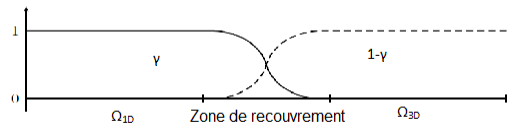
Figure 2.1-a weighting functions in the Harlequin framework

This weighting makes it possible to avoid taking energy into account several times in the same zone and thus allows the user a certain freedom to choose the predominant model. Indeed, it allows you to put weight on the model you want to express.

In the Arlequin framework, as soon as heterogeneous models are coupled, it is recommended to discretize the Lagrange multipliers on the rough model in space. This makes it possible to avoid the phenomenon of digital locking and, therefore, to allow more freedom to each of the models by allowing the fine model to express its wealth. As a result, the finite element space of these Lagrange multipliers is built on the rough model (beam model for this case).

The 3D-Harlequin Beam connection, as developed in Code_Aster, must meet a highly important requirement. Indeed, the 1D and 3D meshes must be « hierarchically compatible », in the sense that all the 3D elements are included in the cylindrical space of the 1D element facing each other (no 3D elements straddling two beam elements). The only constraint that is imposed on the user therefore consists in making an effort when developing the mesh, which is not a bad thing because the final model will be better controlled.

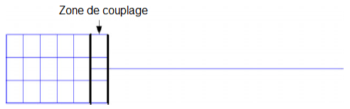
Figure 2.1-b schematic representation of a connection of a mixed 1D-3D cantilever beam model with « hierarchical meshes »

The Arlequin method is used here to connect two 1D and 3D models (junction operation). Consequently, the coupling zone corresponds to the bonding zone. The management of weights to ensure the partition of the unit in the free zone (Harlequin conditions) is managed by the user.

As it is an L2 coupling, it is sufficient to impose the weighting coefficients in the definition of the materials relating to the various free and adhesive zones.

Note:

A general procedure for managing incompatible meshes would be very cumbersome and expensive to program, it would require complicated management of weighting functions in the bonding area as well as an intersection or division into sub-elements of 1D and 3D meshes in order to manage the integration of coupling terms.

2.2. Ratings

Note:

• \(\Omega\) the coupling zone

• \({\mathrm{u}}_{\mathrm{1D}}\) and \({\mathrm{u}}_{\mathrm{3D}}\) the displacement fields corresponding to the 1D beam and 3D models

• \(\lambda\) the Lagrange multiplier associated with the 1D domain

• \(\text{M}\) the classic girder stiffness matrix

2.3. Expression of the Harlequin connection condition

The L2 coupling equation in a continuous medium is written as:

\({\mathrm{\int }}_{\Omega }\lambda \text{:}({\mathrm{u}}_{\mathrm{1D}}\mathrm{-}{\mathrm{u}}_{\mathrm{3D}})\text{d}\Omega \mathrm{=}{\mathrm{\int }}_{\Omega }\lambda \text{:}{\mathrm{u}}_{\mathrm{1D}}\text{d}\Omega \mathrm{-}{\mathrm{\int }}_{\Omega }\lambda \text{:}{\mathrm{u}}_{\mathrm{3D}}\text{d}\Omega\) eq 2.4-1

\(\lambda\) and \({\mathrm{u}}_{\mathrm{1D}}\) have exactly the same type of degrees of freedom and the same type of shape functions because they are defined in the same space as the kinematically admissible fields. In fact, for a 1D element of the Lagrange multiplier, a 1D beam element corresponds.

It is assumed, for simplicity, that the axis of the beam is along X.

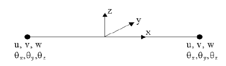
Figure 2.3-a schematic representation of a beam element with 6 degrees of freedom

So, beam-type displacement is classically written as follows:

\(\mathrm{\{}\begin{array}{cccc}u\mathrm{=}u(x)& +z{\theta }_{y}(x)& \mathrm{-}y{\theta }_{z}(x)& +0\\ v\mathrm{=}0& +0& +v(x)& \mathrm{-}(z\mathrm{-}{z}_{c}){\theta }_{x}(x)\\ w\mathrm{=}0& +w(x)& +0& +(y\mathrm{-}{y}_{c}){\theta }_{x}(x)\end{array}\)

The Lagrange multiplier will then be written according to a beam kinematics as follows:

\(\mathrm{\{}\begin{array}{cccc}{\lambda }_{u}\mathrm{=}{\lambda }_{u}(x)& +z{\lambda }_{{\theta }_{y}}(x)& \mathrm{-}y{\lambda }_{{\theta }_{z}}(x)& +0\\ {\lambda }_{v}\mathrm{=}0& +0& +{\lambda }_{v}(x)& \mathrm{-}(z\mathrm{-}{z}_{c}){\lambda }_{{\theta }_{x}}(x)\\ {\lambda }_{w}\mathrm{=}0& +{\lambda }_{w}(x)& +0& +(y\mathrm{-}{y}_{c}){\lambda }_{{\theta }_{x}}(x)\end{array}\)

On a 1D element marked E1d, the first 1D-1D coupling term is written in the same 1D space:

\({\mathrm{\int }}_{{\text{e}}_{\mathrm{1D}}}\lambda \text{:}{\mathrm{u}}_{\mathrm{1D}}\text{d}\Omega \mathrm{=}{\left\{\lambda \right\}}^{t}{\text{C}}_{\mathrm{1D}\mathrm{-}\mathrm{1D}}\left\{{u}_{\mathrm{1D}}\right\}\mathrm{=}{\left\{\lambda \right\}}^{t}\text{M}\left\{{u}_{\mathrm{1D}}\right\}\) eq 2.4-2

where \(\left\{\lambda \right\}\) is the vector of the 12 degrees of freedom of the Lagrange multiplier and \(\left\{{u}_{\mathrm{1D}}\right\}\) is the vector of the 12 degrees of freedom of the beam elements:

\(\left\{{u}_{\mathrm{1D}}\right\}\mathrm{=}({u}^{1},{v}^{1},{w}^{1},{{\theta }_{x}}^{1},{{\theta }_{y}}^{1},{{\theta }_{z}}^{1},{u}^{2},{v}^{2},{w}^{2},{{\theta }_{x}}^{2},{{\theta }_{y}}^{2},{{\theta }_{z}}^{2})\)

\(\left\{\lambda \right\}\mathrm{=}({\lambda }_{u}^{1},{\lambda }_{v}^{1},{\lambda }_{w}^{1},{\lambda }_{{\theta }_{x}}^{1},{\lambda }_{{\theta }_{y}}^{1},{\lambda }_{{\theta }_{z}}^{1},{\lambda }_{u}^{2},{\lambda }_{v}^{2},{\lambda }_{w}^{2},{\lambda }_{{\theta }_{x}}^{2},{\lambda }_{{\theta }_{y}}^{2},{\lambda }_{{\theta }_{z}}^{2})\)

In the particular case of L2 coupling, the matrix \({\text{C}}_{\mathrm{1D}\mathrm{-}\mathrm{3D}}\) is equal to the conventional mass matrix of a beam element.

Still on a 1D element noted E1d, the second 1D-3D coupling term is written in the same 1D space:

\(\mathrm{-}{\mathrm{\int }}_{{\text{e}}_{\mathrm{1D}}}\lambda \text{:}{\mathrm{u}}_{\mathrm{3D}}\text{d}\Omega \mathrm{=}\mathrm{-}{\left\{\lambda \right\}}^{t}{\text{C}}_{\mathrm{1D}\mathrm{-}\mathrm{3D}}\left\{{u}_{\mathrm{3D}}\right\}\) eq 2.4-3

and \(\left\{{u}_{\mathrm{3D}}\right\}\) is the vector of the (3 x \({N}_{\mathit{no3D}}\)) degrees of freedom of the 3D elements (\({N}_{\mathit{no3D}}\) being the number of nodes in the 3D element):

\(\left\{{u}_{\mathrm{3D}}\right\}\mathrm{=}({u}^{1},{v}^{1},{w}^{1},\text{...},{u}^{{N}_{\mathit{no3D}}},{v}^{{N}_{\mathit{no3D}}},{w}^{{N}_{\mathit{no3D}}})\)

The process of constructing the \({\text{C}}_{\mathrm{1D}\mathrm{-}\mathrm{3D}}\) matrix on the 3D fine model is more delicate than that of the rough Beam model. The complexity of this coupling lies in the coexistence of two fields belonging to different spaces. It is obtained by considering all the 3D elements contained in the cylindrical space of the 1D element.

\({\text{C}}_{\mathrm{1D}\mathrm{-}\mathrm{3D}}\mathrm{=}\mathrm{\sum }_{k\mathrm{=}1}^{{N}_{\mathit{el3D}}}{\text{C}}_{\mathrm{1D}\mathrm{-}\mathrm{3D}}^{k}\)

It is recalled that, by constructing the mesh itself, all the 3D elements must be included in this space. These elements are determined by a matching procedure (relationship graph) which consists in projecting their barycenters into the geometric support of the associated 1D element (projection of a point on a segment).

For each 3D element number k (k ranging from 1 to Nel3D), the matrix \({\text{C}}_{\mathrm{1D}\mathrm{-}\mathrm{3D}}^{k}\) is calculated in the following way:

\({\text{C}}_{\mathrm{1D}\mathrm{-}\mathrm{3D}}^{k}\mathrm{=}\mathrm{\sum }_{g\mathrm{=}1}^{\mathit{Nbgauss}}{\mathrm{W}}^{g}{\mathrm{B}}_{\mathrm{1D}}^{gt}({\xi }_{\mathrm{1D}}){\mathrm{G}}^{g}{\mathrm{B}}_{\mathrm{3D}}^{g}({\xi }_{\mathrm{3D}},{\eta }_{\mathrm{3D}},{\zeta }_{\mathrm{3D}})\text{det}({\mathrm{J}}^{\mathrm{g}})\)

with G the passage matrix Reference element — Physical element, containing zeros and elements of the Jacobian inverse calculated at the Gauss point g.

The \({\mathrm{B}}_{\mathrm{1D}}^{g}\) matrix is 3x in size (3x number of nodes in the 1D element). Its terms are calculated at the Gauss points of the 1D elements.

\({\mathrm{B}}_{\mathrm{1D}}^{g}\mathrm{=}\left[\begin{array}{cccccccccccc}{N}_{1}^{p}& y{\xi }_{5}& z{\xi }_{5}& 0& z{\xi }_{6}& \mathrm{-}y{\xi }_{6}& {N}_{2}^{p}& y{\xi }_{7}& z{\xi }_{7}& 0& z{\xi }_{8}& \mathrm{-}y{\xi }_{8}\\ 0& {\xi }_{1}& 0& \mathrm{-}z{N}_{1}^{p}& 0& \mathrm{-}{\xi }_{2}& 0& {\xi }_{3}& 0& \mathrm{-}z{N}_{2}^{p}& 0& \mathrm{-}{\xi }_{4}\\ 0& 0& {\xi }_{1}& y{N}_{1}^{p}& {\xi }_{2}& 0& 0& 0& {\xi }_{3}& y{N}_{2}^{p}& {\xi }_{4}& 0\end{array}\right]\)

where x, y and z are the local variables of the 1D element, \({N}_{1}^{p}\) and \({N}_{2}^{p}\) are the shape functions for traction-compression-torsional, \({\xi }_{\mathrm{1...8}}\) are the flexure shape functions of the beam (cf. document [r3.08.01] by Code-Aster).

The \({\mathrm{B}}_{\mathrm{3D}}^{g}\) matrix is 3x in size (3x number of nodes in the 3D element). For example, the matrix \({\mathrm{B}}_{\mathrm{3D}}^{g}\) associated with the tetrahedron linear volume element (TETRA4) is written as:

\({\mathrm{B}}_{\mathrm{3D}}^{g}\mathrm{=}\left[\begin{array}{cccccccccccc}{N}_{1}& 0& 0& {N}_{2}& 0& 0& {N}_{3}& 0& 0& {N}_{4}& 0& 0\\ 0& {N}_{1}& 0& 0& {N}_{2}& 0& 0& {N}_{3}& 0& 0& {N}_{4}& 0\\ 0& 0& {N}_{1}& 0& 0& {N}_{2}& 0& 0& {N}_{3}& 0& 0& {N}_{4}\end{array}\right]\)

The variables x, y, z as well as the shape functions and their derivatives are calculated at the Gauss point g of the 3D element. So, for example, we have:

\(\begin{array}{c}x\mathrm{=}\mathrm{\langle }N\mathrm{\rangle }\left\{{x}_{n}\right\},{u}_{x}\mathrm{=}\mathrm{\langle }N\mathrm{\rangle }\left\{{u}_{n}\right\}\\ y\mathrm{=}\mathrm{\langle }N\mathrm{\rangle }\left\{{y}_{n}\right\},{u}_{y}\mathrm{=}\mathrm{\langle }N\mathrm{\rangle }\left\{{v}_{n}\right\}\\ z\mathrm{=}\mathrm{\langle }N\mathrm{\rangle }\left\{{z}_{n}\right\},{u}_{z}\mathrm{=}\mathrm{\langle }N\mathrm{\rangle }\left\{{w}_{n}\right\}\end{array}\)

where:

• xn, yn, and zn are the coordinates of the nodes of the 3D element,

• one, ven, and wn are the degrees of freedom associated with the nodes of the 3D elements,

• \(\mathrm{\langle }N\mathrm{\rangle }\) is the vector containing all the shape functions of the 3D element according to the order of the 3D nodes (cf. document r3.01.01 from Code-Aster).

For each Gauss point with coordinates \(({\xi }_{\mathrm{3D}},{\eta }_{\mathrm{3D}},{\zeta }_{\mathrm{3D}})\) in the 3D reference element, we introduce its physical representation in the form of the following interpolated \((\stackrel{ˉ}{X},\stackrel{ˉ}{Y},\stackrel{ˉ}{Z})\) coordinates:

\(\stackrel{ˉ}{X}\mathrm{=}\mathrm{\sum }_{i\mathrm{=}1}^{{N}_{\mathit{el3D}}}{N}^{i}{x}^{i}({\xi }_{\mathrm{3D}},{\eta }_{\mathrm{3D}},{\zeta }_{\mathrm{3D}})\)

\(\stackrel{ˉ}{Y}\mathrm{=}\mathrm{\sum }_{i\mathrm{=}1}^{{N}_{\mathit{el3D}}}{N}^{i}{y}^{i}({\xi }_{\mathrm{3D}},{\eta }_{\mathrm{3D}},{\zeta }_{\mathrm{3D}})\)

\(\stackrel{ˉ}{Z}\mathrm{=}\mathrm{\sum }_{i\mathrm{=}1}^{{N}_{\mathit{el3D}}}{N}^{i}{z}^{i}({\xi }_{\mathrm{3D}},{\eta }_{\mathrm{3D}},{\zeta }_{\mathrm{3D}})\)

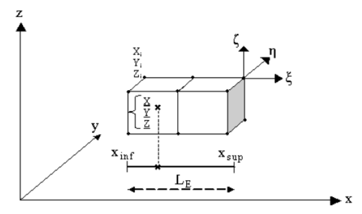
Figure 2.3-b operation to locate the Gauss points of a 3D element in the single beam element that is paired with it

To simplify the illustration, we assume that the axis of the beam is along X. For each Gauss point of the 3D element, we introduce its projection onto the single real 1D element that is paired with it as follows:

\({\stackrel{ˉ}{\xi }}_{\mathrm{1D}}\mathrm{=}\frac{\stackrel{ˉ}{X}\mathrm{-}{X}_{\mathit{inf}}}{\text{Le}}\)

The coordinates of the projection in the other two directions of the thickness of the beam are given by \(y\mathrm{=}\stackrel{ˉ}{Y}\) and \(z\mathrm{=}\stackrel{ˉ}{Z}\).

This technique makes it possible to discretize the Lagrange multiplier on the beam elements and to calculate the integrals in the expressions of the coupling matrices \({\text{C}}_{\mathrm{1D}\mathrm{-}\mathrm{3D}}^{k}\). Thus, for each 3D element, the matrix \({\text{C}}_{\mathrm{1D}\mathrm{-}\mathrm{3D}}^{k}\) is calculated as follows:

\({\text{C}}_{\mathrm{1D}\mathrm{-}\mathrm{3D}}^{k}\mathrm{=}\mathrm{\sum }_{g\mathrm{=}1}^{\mathit{Nbgauss}}{\mathrm{W}}^{g}{\mathrm{B}}_{\mathrm{1D}}^{gt}({\stackrel{ˉ}{\xi }}_{\mathrm{1D}}){\mathrm{G}}^{g}{\mathrm{B}}_{\mathrm{3D}}^{g}({\xi }_{\mathrm{3D}},{\eta }_{\mathrm{3D}},{\zeta }_{\mathrm{3D}})\text{det}({\mathrm{J}}^{\mathrm{g}})\)

where the beam-like shape functions are interpolated to the parametric coordinates of the projected points obtained.

2.4. Implementation of the connection method

For each Arlequin connection, the user must define the following operands under the 3D_ POU_ARLEQUIN option of the LIAISON_ELEM keyword:

The 3D group of elements in the collage area (keyword GROUP_MA_1)

The 1D group of elements in the collage area (keyword GROUP_MA_2)

The CHAM_MATER concept defining materials (serving to ensure the partition of the unit)

The concept CARA_ELEM defining the elementary characteristics used to calculate the coupling matrices \({\text{C}}_{\mathrm{1D}\mathrm{-}\mathrm{1D}}\) and \({\text{C}}_{\mathrm{1D}\mathrm{-}\mathrm{3D}}\)

For each beam element, Code_aster calculates the linear relationships resulting from writing the assembled coupling matrices [éq 2.4-1]. These kinematic relationships link:

• the 12 degrees of freedom of the two nodes of the beam element,

with the degrees of freedom of the nodes of**all* the elements paired with the beam element.

Finally, the resulting linear relationships will be dualized, like all linear relationships resulting from the keyword LIAISON_DDL in AFFE_CHAR_MECA, for example.

[1]

In practice, the Code_Aster user will be asked to provide hierarchical meshes.