6. Calculation of contact contributions#

For a contact problem treated with the continue method, the resolution is done with 5 loops nested in the operator STAT_NON_LINE [U4.51.03]:

loop on the load steps,
geometric buckle,
loop on the friction thresholds,
active constraint loop,
Newton iterations.

To understand the general functioning of the STAT_NON_LINE operator, we strongly recommend reading the document [D9.05.01]. FIG. 5 represents the call tree of this operator for the specific case of an X- FEM contact problem. The locations of the loops mentioned above can thus be found in this figure.

Figure 5 also makes it possible to identify where the major computer developments carried out for the large swings with X- FEM approach are located, namely:

the geometric update call tree (shown in Figure 6),
the call tree for calculating the touch-friction contributions (shown in Figure 7).
the call tree for updating contact statuses (shown in Figure 8),

Below is an example of calling the STAT_NON_LINE operator for an X- FEM analysis:

UTOT1 = STAT_NON_LINE (MODELE = MODELEK,

CHAM_MATER = CHAMPMAT,

EXCIT =( _F (CHARGE = CTXFEM,),

_F (CHARGE = CHXFEM,),

_F (CHARGE = CH1, FONC_MULT = VAR1),),

COMPORTEMENT =_F (RELATION =” ELAS “,

GROUP_MA =” SURF “,),

INCREMENT =_F (LIST_INST =L_ INST,),

CONVERGENCE =_F (ITER_GLOB_MAXI =8,

RESI_GLOB_MAXI =1E-06,),

SOLVEUR =_F (METHODE =” MUMPS “,

PCENT_PIVOT =500,),

ARCHIVAGE =_F (CHAM_EXCLU =” VARI_ELGA “,),

INFO =1,);

The description of Fortran routines:

OP0070 - only one change here: the call for the routine of zeroing contact Lagrangians. For the case X- FEM, the routine XMISZL does the same thing as the old routine MISAZL does in the standard case of contact with the continuous method.

NMCTGE — hat routine that starts the calculation of the geometry of the contact facets (XREACG) and the matching (XAPPAR).

XREACG — a new routine that updates the position of the intersection points forming the contact facets. We use SD MODELE//”. TOPOFAC .OE”, containing the initial position of the intersection points, to calculate SD MODELE//”. TOPOFAC .GE”, and MODELE//”. TOPOFAC .GM”, by calling XGECFI. These last 2 SDs correspond respectively to the updated coordinates of the slave and master sides.

XGECFI — starts the calculation of the new geometry of the contact facets (slave and master). We go through an elementary calculation (TE0519 with the option « GEOM_FAC « ).

TE0519 — calculate the new geometry of the intersection points forming the contact facets (slave and master). We go back with the initial geometry of the facets, stored in MODELE//”. TOPOFAC .OE”. We come out with the updated slave and master geometries in MODELE//”. TOPOFAC .GE” and MODELE//”. TOPOFAC .GM”. The update is performed at each start of the geometric loop. It is then used to match the slave contact points to the master stitches.

XAPPAR — new routine for pairing in case X- FEM. It is a complex routine, which in turn calls for other routines (see the call tree). The principle is to loop on the contact zone, then on the slave meshes, then on the contact facets of the slave mesh, and finally on the contact points belonging to the contact facet. For each contact point we fill in CHAR//”. CONTACT. TABFIN “with information about the slave touchpoint and the master mesh found, in order to create the pairing. Remember: there must be as many late stitches as there are contact points.

MMGAUS — calculate the reference coordinates of the integration point in the contact facet.

XCOPCO — new routine called by XAPPAR to calculate the real COordonnées of a Point of COntact based on the knowledge of its reference coordinates (determined with the old MMGAUS routine) and the coordinates of the intersection points of the contact facet of the slave mesh.

XMREPT — new routine for REcherche from the intersection point on the master side, closest to the current contact point. It provides a certain amount of information on this intersection point: its local number, the local number of the edge (or of the node if the crack passes through a node) that contains it, and the global number of the mesh that contains it. This information will feed the search for the project on the master lip. Note that this step makes it possible to restrict the number of facets onto which the slave point will be projected in XMREMA, in order to improve performance. In some cases (even in classical finite elements) this selection is too restrictive and leads to false results. This approach should be reviewed.

XMREMA — new routine for REchercher the closest MAille master knowing the closest master intersection point to the contact point and to then do the projection. We leave here with essential information on the project and the master cell (reference coordinates, global number of the master cell, the base tangent to the projection point, information on the projection outside the master surface, etc.). In 2D, the only contact facet associated with the master mesh is always a SEG2. In 3D, the associated master facet is always a TRI3, but since there are several facets per mesh, it is also important to determine the facet number. In the case of multi-crack, the local number of the crack corresponding to the contact zone in the master element is also determined. This number was previously determined in XMACON and stored in SDCHAR//”. CONTACT. MAESCL “.

MMPROJ — old routine of the FEM contact method, which projects a contact point onto a given mesh. For the X- FEM method, this mesh is « fictional » and defined by the updated coordinates of the intersection points defining the master contact facet.

XMCOOR — new routine that calculates the reference coordinates of a contact point in the parent mesh (slave or master) knowing the reference coordinates of this point in the contact facet, and the reference coordinates of the points of the contact facet in the parent mesh.

XMRLST — new routine that calculates, from the tangent level set, the square root of the distance to the bottom of the crack for the slave and master integration points. This is useful when the element is enriched by Crack Tip functions.

XPIVIT — new routine that determines if the integration point is vital or not. We see if the contact point is on an edge, and if so, we give it the status of the edge in question (status stored in TOPOFAC .AI). We leave here with the « vital point » or « non-vital point » information, as well as the group number and edge number of this group if the contact point is located on an edge belonging to a group of connected edges.

NMCTCL — routine hat for preparing data in order to start calculating contact contributions. Changes have been made in order to launch the creation of the LIGREL (LIste of GRoupes of ELéments of the same type) containing hybrid contact elements (routine XMLIGR) and contact cards (routine XMCART) by the creation of the (of of of the same type).

XMLIGR — new routine for creating LIGREL for new late contact elements. This is where the contact elements are created by the association between a slave mesh and a master mesh. We then put them in GREL and then in LIGREL. The routine is similar to the old routine MMLIGR. 2D late meshes of type QU8QU4 and TR6TR3 relate to the old formulation (P1-P2). They will be absorbed later. For the new formulation, 2D late meshes QU4QU4, TR3TR3,,, QU4TR3 and TR3QU4 are available in order to process the linear contact (P1-P1) as well as the QU8QU8 and TR6TR6 meshes for the semi-quadratic (P2-P1). In 3D only meshes HE8HE8, PE6PE6 and TE4TE4 are available and contact treatment is only possible linearly (P1-P1). Finally, to treat the different types of x-fem elements, each late mesh described above (only for P1-P1) is associated with several late elements (specificity of X-fem FEM). Thus, in addition to element \(H-H\), we have elements \(H\mathrm{-}\mathit{HCT}\), \(\mathit{HCT}\mathrm{-}H\), \(\mathit{HCT}\mathrm{-}\mathit{HCT}\) and finally \(\mathit{CT}\) (which is all alone because it is treated in small slips for the moment) to treat the large slip contact at the crack point. In the case of multi-cracking, it is also possible to match elements that do not have the same number of Heaviside degrees of freedom. Thus, it is also possible to process the elements \(H-{H}_{2}\), \(H-{H}_{3}\), \(H-{H}_{4}\),, \({H}_{2}-H\),, \({H}_{2}-{H}_{2}\),, \({H}_{2}-{H}_{3}\), \({H}_{2}-{H}_{4}\), \({H}_{3}-H\), \({H}_{3}-{H}_{2}\), \({H}_{3}-{H}_{3}\), \({H}_{3}-{H}_{4}\) \({H}_{4}-H\) \({H}_{4}-{H}_{2}\) , \({H}_{4}-{H}_{3}\), \({H}_{4}-{H}_{4}\). Since the number of types of Multi-Heaviside elements is high (because they must also be generated for each type of mesh), the libraries of late Multi-Heaviside elements were generated using a Python script.

XMELEL — provides information about the late contact item. This routine works for all of the items listed in XMLIGR. Given the large number of elements, this routine returns several pieces of information on the late element (slave and master mesh type, slave and master element type, modeling type) in order to reconstruct the element type dynamically in XMLIGR.

XMCART — routine for creating contact cards (fields that contain information about contact items). We use cards but we would have to reprogram all this to use CHAM_ELEM instead as in the classic case (routine MMCHML). In the classical case, only one field is created. In X- FEM we create several maps because we must provide elementary calculation with information on the topology of the X- FEM elements. In addition, some of this information must be provided both for the slave mesh and also for the master mesh. We create the map RESOCO//”. XFPO “, which is equivalent to CHAM_ELEMRESOCO//”. CHML “in the classic case; the RESOCO//” card. XFST “which stores the enrichment statuses of slave and master mesh nodes; the RESOCO//” map. XFPI “containing the positions of the slave intersection points in the reference coordinates; the RESOCO//” map. XFAI “containing information on slave intersected edges; map RESOCO//”. XFCF “containing information on the connectivity of the slave contact facets; in the case where at least one of the master or slave elements is multi-cracked, the 2 additional cards are added: RESOCO//”. XFHF “which contains the value of the Heaviside functions corresponding to the enrichments on the master and slave sides and RESOCO//”. XFPL “which contains the place of the Lagrangians associated with the nodes in the matrix.

NMELCM — routine to start calculating elementary contact friction matrices. It is common to continuous contact approaches (FEM, X- FEM HPP, X- FEM GG).

NMELCV — routine to start calculating the second friction contact members. It is common to continuous contact approaches (FEM, X- FEM HPP, X- FEM GG).

TE0366 — new elementary calculation routine for the contributions of friction contact to the stiffness matrix, in the large slipswith X- FEM approach. A large number of routines (presented below) are called here. Most are also referred to in TE0367 and TE0363.

TE0367 - new elementary calculation routine for the contributions of friction contact to the second limb, in the large slips approach with X- FEM *.

XMELET — new routine for retrieving information about the current contact element. We go back with the name of the late element. We come out with the names of the slave and master cells; the number of the contact facet; the numbers of ddls, slaves and masters, of the contact facet; the total number of ddls; the information on the type of formulation (middle nodes or vertex nodes).

XMPINT — new routine for calculating the real coordinates of the intersection points constituting the contact facet.

XTFORM — compute the shape functions and their derivatives of the integration point using the parametric coordinates in the parent element. It is called by the numbers TE0366 and TE0367, the derivatives of the shape functions are then used to calculate the Jacobian of the contact point in XMMJAC.

XLACTI — calculate the active status or not of contact Lagrangians. A node is active if it belongs to a cut edge or is directly cut by the crack.

XMOFFC — distributes the shape functions of the nodes where the Lagrangians are to be eliminated on the active nodes.

XMMJAC — new routine used to calculate the Jacobian for the point of contact.

MMNORM — old routine for calculating the outgoing normal at the projected point of contact. Attention, in 3D we do not call MMNORM, because the facets are oriented in the other direction for the contact method X- FEM compared to the contact method FEM.

XTCALN — calculate the normal vector.

PROVEC — old routine that is used to make the vector product of tangent vectors to obtain the normal vector in 3D.

NORMEV — old routine that normalizes a vector. It is used to normalize the normal vector in 3D, but it is also called to project the friction vector onto the unit ball in the sliding case of friction.

XOULA — routine specific to X- FEM, which is used for the connectivity of contact ddls. It is no longer used for the formulation at vertex nodes.

XPLMA2 — new routine that provides the place of a contact ddl in the elementary stiffness matrix, corresponding to the late elements X- FEM. The corresponding routine in HPP is XPLMAT.

XTLAGM — calculate the contact and friction Lagrangians for the contact point.

XTLAGC — calculate the contact Lagrangian for the contact point

XTLAGF — calculate the Lagrangian friction for the contact point

XTDEPM — calculate the displacement increments since the previous time step of the slave contact point and the sound projected onto the master facet.

XMMJEU — new routine called by TE0366 and TE0367 to calculate the game between the contact point and the projected sound. During Newton iterations, we have access to the total displacements of the previous time step (idepl) and to the increments of movements from the previous time step to the current Newton (idepm). The position is therefore calculated by making initial geometry + total displacement of the previous time step + increment up to the current Newton.

XMMJEC — new routine called by TE0363 to calculate the game between the contact point and the projected sound. When the contact statuses are updated, we have access to total movements (idepl): the position is therefore calculated by making initial geometry + total displacement.

TTPRSM — old routine that calculates \({g}_{\tau }\), \(∣∣{g}_{\tau }∣∣\), and \(\mathrm{[}{P}_{\tau }\mathrm{]}\).

XMMAA1 — new routine for calculating the terms \({A}_{u}\), \(A\) and \({A}^{T}\) (case with contact) of the contact stiffness matrix. The expressions for the contact friction terms in the stiffness matrix and in the second member are given in the documentation [R5.03.53].

XMMAA0 — new routine for calculating terms due to contact modeling in the stiffness matrix (non-contact case).

XMMAB0 - new routine for calculating terms due to contact modeling in the stiffness matrix (case of frictionless contact).

XMVEC1 - new routine for calculating the terms of the second member (case with contact).

XMVEC0 - new routine for calculating the terms of the second member (non-contact case).

XMMAB2 - new routine for calculating the terms \(\mathit{Bu}\), \(B\), \(\mathit{BT}\) and \(F\) in the friction stiffness matrix (case of sliding friction contact).

MKKVEC — old routine that applies a transformation to a vector. This routine is called by XMMAB2 and is useful for calculating friction matrices dependent on \(K({g}_{\tau })\).

XMMAB1 - new routine for calculating the terms \(\mathrm{Bu}\), \(B\), \(\mathrm{BT}\) in the friction stiffness matrix (case of adherent friction contact).

XMMAB0 - new routine for calculating the friction term \(F\) in the friction stiffness matrix (case of frictionless contact or case without contact).

XMVEF1 - new routine for calculating the friction terms \({L}^{\mathrm{1frott}}\) and \({L}^{\mathrm{3frott}}\) for the second limb (case of friction contact).

XMVEF0 - new routine for calculating the friction term \({L}^{\mathrm{3frott}}\) for the second limb (non-contact cases and frictionless cases).

XTEDD2 — new routine that eliminates Heaviside and Crack Tip degrees of freedom in excess for contact contributions in large X- FEM slides. It also eliminates excess contact ddls.

Figure 5. The STAT_NON_LINE operator call tree for dealing with a contact problem in large swings with XFEM.

Figure 6. The call tree during a geometric rematch for a large-scale contact problem with X- FEM.

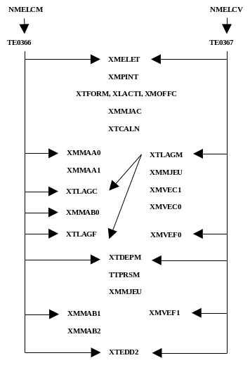
Figure 7. The call tree for calculating contact contributions in the matrix and the second member for a large-scale contact problem with X- FEM.