4. General algorithm#
The process is standardized as much as possible, for each loop level:
Evaluation of convergence by calling nmcvg routines;
Action following the loop situation by calling the nmact routines;
4.1. Global reads and initializations#
The op0070 routine manages the global algorithm and is divided into three parts:
Reading and initializing data;
Loop over the time steps;
Post-treatments;
Global error management;
Archiving;
For reading and initializing data, reference should in particular be made to information relating to SD management (§ 2). All the initializations made at this level will be valid for the entire calculation. The main initialization routine is nminit. Here are the operations planned in this routine:
Initialization operations in nminit |
Routine |
Creating the matrix profile and the SDNUME |
nmnume |
Creating hat variables |
nmchap |
Creating the vector of activated functionalities list_func_acti |
nmfonc |
Creating vectors in hat variables |
nmcrch |
Creation of the management data structure |
nmdopi |
Duplication NUME_DDLpour SDNUME |
nmpro2 |
Preparing map COMPOR (transformation into CHAM_ELEM_S) |
nmdoco |
Creating SDDISCet SDOBSE |
diinit |
Initializing command variables |
nmcrvv |
Pre-calculation of the MATR_ELEM constants during the calculation |
nminmc |
Pre-calculation of VECT_ELEM and VECT_ASSE constants during the calculation |
nminvc |
Creating the SDCRIT |
nmcrcv |
Initialization of the calculation by substructuring |
nmlssv |
Creating the SD for loading FORCE_SOL |
nmexso |
Calculating the initial acceleration |
accel0 |
Creating the SDCONV |
nmcrcg |
Initializing NL_DS_Print |
nminim |
Pre-calculation of the MATR_ASSE constants during the calculation |
nminma |
Conducting an initial observation |
nmobsv |
Creation of SD RESULTAT (EVOL_NOLI) |
mnoli |
Creation of the size table (for ERRE_THM) |
cetule |
Calculation of the initial second member for multi-step schemes in dynamics |
nmihht |
The general algorithm of op0070 is summarized on the flowchart ().
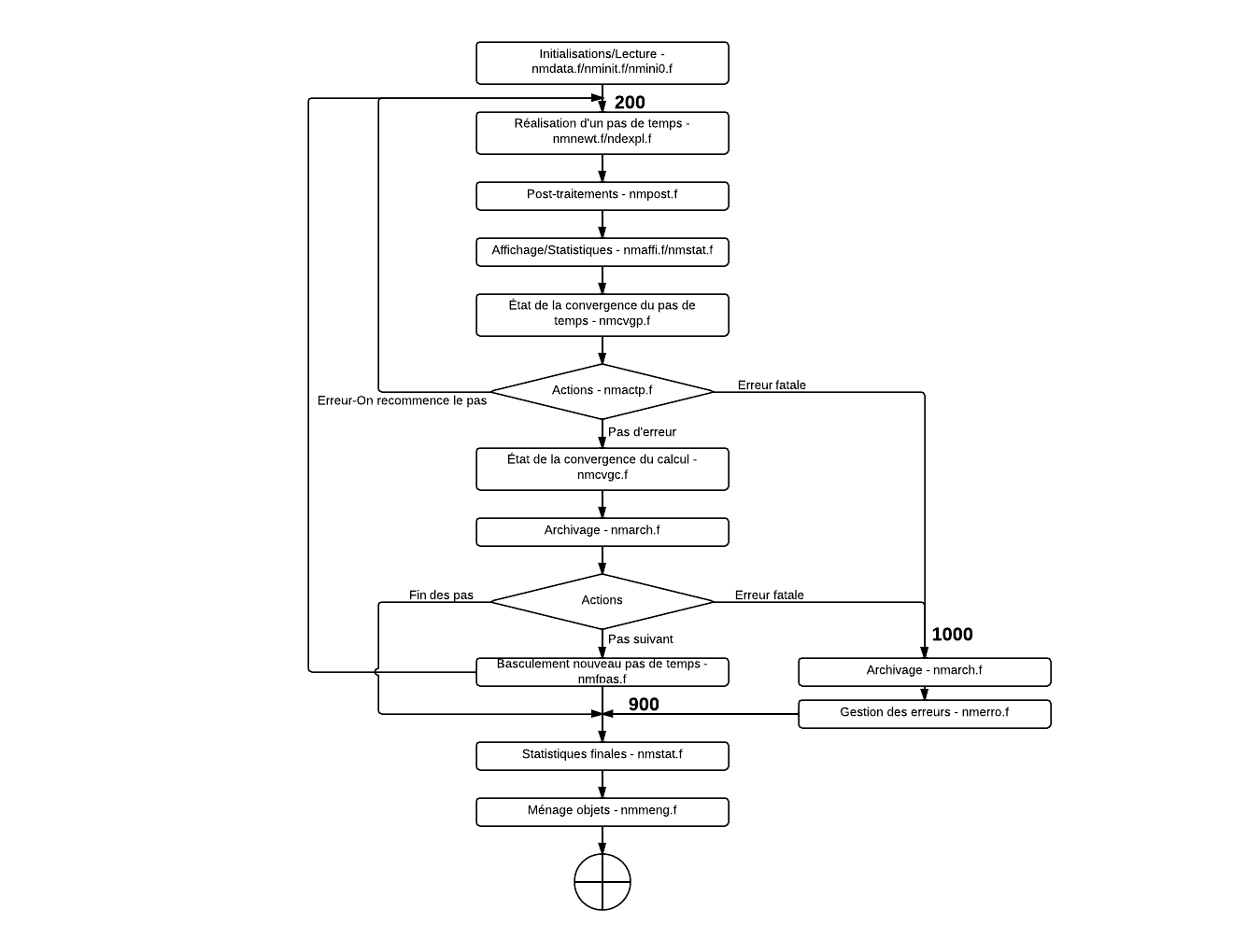
|
Figure 1: General flowchart of op0070 |
4.2. Completion of a time step#
A time step uses several levels of nested loops:
Fixed point loops, used exclusively for contact (up to three loop levels);
A loop over Newton’s iterations. A Newton process contains an Euler prediction and Newton corrections;
The general nmnewt algorithm is summarized in the flowchart ().
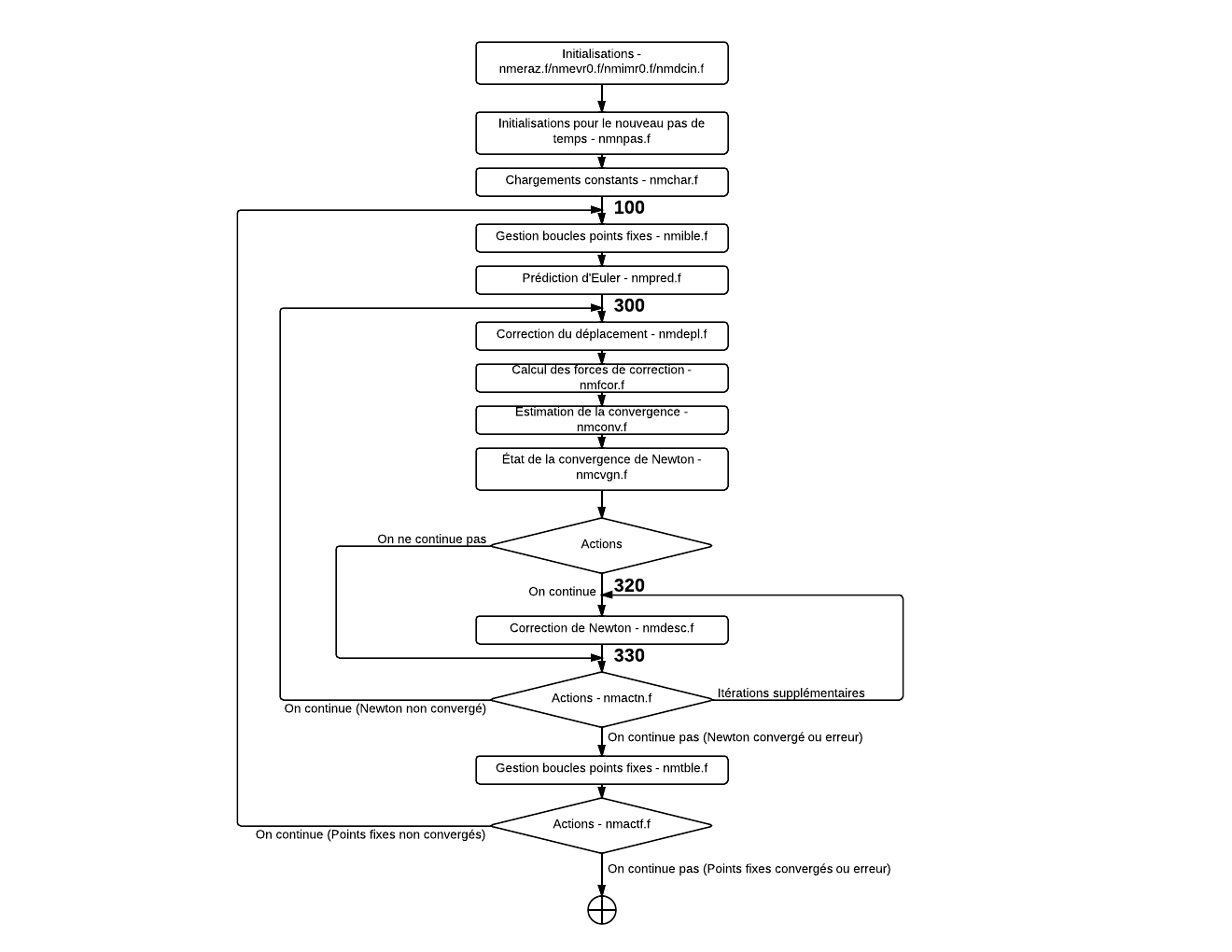
|
Figure 2: General organization chart of NMNewt |
4.2.1. Step initializations#
Each time step is initialized by a series of routines:
The routines nmeraz, nmevr0 take care of initializing event management;
The nmdcin routine verifies that the cutting of the time step is correct (checking the number of cutting levels from one time step to the next);
The most important routine is the nmnpas routine. It carries out the following operations:
The nmimr0 and nminin routines initialize the display, in particular the convergence table (which makes it possible to vary the nature of this one from one time step to another);
The nmvcre routine prepares the command variables for the current time step;
The cumulative displacement increment since the start of the time step is initialized to zero (vector DEPDEL, see § 2.4.1.6). Attention the initialization is special because of the consideration of large rotations;
We initialize all the data for the dynamics, in particular the various coefficients (see § 2.4.2.17) in ndnpas;
We initialize various information for Newton-Krylov and the contact (cfinit, mmapin and mnkft routines);
4.2.2. Euler’s prediction#
Euler prediction is an estimate of the displacement increment by linearizing the problem with respect to time. There are several methods and several types of matrix that can be used. The actual calculation is carried out in the nmpred routine (and its -pretty- daughters), using the principles established in § 5.
4.2.3. Update fields#
The fields are updated in the nmdepl routine. This update consists in modifying the solution vectors (displacements, speeds and accelerations), possibly taking into account:
Linear research without control;
The search for \(\eta\) for piloting with or without linear research;
Contact (discrete formulation) or unilateral relationships;
Here are the phases:
Recalculation of external forces, nmfext routine;
Conversion of the solution increments DEPSO1 and DEPSO2 (see § 2.4.1.6), resulting from the resolution of the linear system, to the displacement/speed/acceleration increments (taking into account the schema change coefficients), via the nmincr routine;
Calculation, linear research and control, routines: nmreli, nmpich and nmrepl;
Update of the descent direction (taking into account the coefficients from linear research and piloting), nmpild routine;
Modification of movements through contact and unilateral connections, through the nmcoun routine;
Updating the solution fields in nmmajc;
Phase 4.2.3 consists in updating the « plus » fields (DEPPLU, VITPLU, ACCPLU) and the cumulative fields (DEPDEL, VITDEL, ACCDEL), taking into account possible large rotations (updating the quaternions) and damage to the nodes.
4.2.4. Correction forces#
Since the displacements have been modified (see § 4.2.3), it is necessary to re-evaluate the variable forces: either the external forces of the « follower » type, or the internal forces and the contact/friction reactions, or the forces related to dynamics (inertia, damping). The set is carried out in the nmfcor routine.
4.2.5. Convergence estimation#
The estimation of Newton’s convergence is a critical moment, which will condition the accuracy of the calculation. All of the estimation is carried out in the nmconv routine. This routine takes care of the calculation of the residues (nmresi), the estimation of their convergence (nmcore). It is therefore in this routine that we will deal with loop <RESI> on balance residues. But we must also take into account the number of iterations of Newton, the case of contact convergence (discrete or continuous formulations), the De Borst method or the IMPLEX method.
Note:
You should be very careful in changing this routine.
4.2.6. Newton correction#
If the process has not converged, a Newton correction is calculated. We therefore perform the calculation of a linear system (see § 5) in the nmdesc routine (as the direction of desc between).
4.2.7. Loop on fixed points#
There are three so-called « fixed point » loops between the loop on the time steps and the loop on the Newton iterations. These loops are used for contact:
Fixed point loop on geometry;
Fixed point loop on friction thresholds;
Fixed point loop on contact statuses;
These three loops are managed by the nmible/nmtble routine duo, via the passage of the variable NIVEAU, which indicates what type of fixed point loop we are currently in.