1. Gprof#
1.1. Building a version with gprof#
To work, gprof needs the sources to have been compiled with the -pg option.
To keep the Code_Aster construction by default (without the gprof options), we use an alias waf_prof (you just need to create a symbolic link for this).
Then, simply include the gprof configuration after setting up the machine to add the necessary options.
On Calibre machines and official servers, the –use-config option is optional in normal times (determined automatically when the env_unstable.sh environment is loaded). Here, we are forced to name it explicitly. So replace XXX with calibre7 or aster5 or…
cd $ HOME /dev/codeaster/src
ln -s waf_variant waf_prof
. /waf_prof configure –use-config= XXX, gprof –prefix=.. /install/prof
. /Waf_prof install
Note
**optimized* mode is in principle preferable for measuring the « true » performance of the code. On the other hand, the* « debug » mode is necessary if we want to know the most consuming lines (then use . /Waf_prof (install_debug) .
We unfortunately observed an inexplicable problem in « debug » mode: the result of the profiling indicated call links between routines that did not exist! However, we can hope that this anomaly does not completely invalidate the rest of the measure.
1.2. Over-cost of instrumentation#
As an example, on the ssnv506c test, the following overall results were obtained:
|
138s |
|
139s |
|
218s |
|
228s |
We note that instrumentation has a negligible cost CPU.
1.3. Executing the instrumentated executable with waf#
To start a test with waf, you can add a line of this type in the.export file to get the gprof file and copy it, for example, to /tmp:
F name /tmp/gmon.out R 0
Then simply launch:. /Waf_prof test -n ssnv506c
See the next paragraph for how to use this gmon.out file.
1.4. Executing the instrumentated executable with astk#
You can also run the study you want to « profile » with the executable instrumentated in astk.
To do this, you must declare the instrumentated version in the list of versions that can be used locally.
In the $ HOME /.astkrc/prefs file, add the line:
to: DEV_PROF: $ HOME /dev/codeaster/install/prof
In astk, all you have to do is select the version named DEV_PROF.
Running the study produces a file (called gmon.out) in the temporary execution directory.
To keep the precious gmon.out file, we add a field in the astk profile of the « name » type and whose value is « … /gmon.out ». We will then retrieve a file with the name gmon.out in the path indicated.
1.5. Exploitation of results#
However, the file produced, at no additional cost, by the instrumentated executable cannot be used directly. You have to run gprof to make it readable (note that it is necessary to specify the name of the instrumentated executable):
gprof $ HOME /dev/codeaster/install/prof/prof/bin/astergmon.out > listing
The analysis therefore consists in analyzing the product listing file.
Attention
You should not be discouraged. For an execution of 30s, as we have already seen, the gprofcommand consumes more than 5 minutes of CPU. The time of gprofdoes not depend too much (a prima facie) on the time of the profiled execution.
The interpretation of the obtained file (listing) is described below. An excellent document describing the entire profiling process is the one written by Jay Fenlason and Richard Stallman: « Gnu gprof The GNU profiler ». It is easily found on the web.
Note
Even if you recompile all Aster sources, the « depth » of performance analysis stops at the libraries that are used when editing links and that were not compiled with « -pg ». This is for example the case with routines*blas. The time consumed in these libraries cannot be traced back to the Code_Aster routines that call them. This defect can be important, for example, if we want to measure the performance of solvers MUMPSou MULT_FRONT because a large part of the time consumed is consumed in routines blas.
1.6. Analyze profiling results#
By default, the file is large. It is possible to limit the display of information by playing with the gprof options. « System times » are indicated in the form of the number of instructions used.
Let’s go into a bit of detail, starting at the end of the file:
Index by function name

[:ref:`401 <401>`] Pyarg_parse [:ref:`591 <591>`] cftabl_ [:ref:`1000 <1000>`] proc_at_0x1213acb50

[:ref:`212 <212>`] pyarg_parseTuple [:ref:`84 <84>`] cftyli_ [:ref:`660 <660>`] proc_at_0x1213ad470

[:ref:`1137 <1137>`] pyarg_parsetupleand [:ref:`310 <310>`] cgmacy_ [:ref:`453 <453>`] proc_at_0x1213ad560

[:ref:`1605 <1605>`] PyBuffer_FromObject [:ref:`79 <79>`] charm_ [:ref:`680 <680>`] proc_at_0x1213aeac0

[:ref:`1256 <1256>`] Py CFunction_Fini [:ref:`476 <476>`] chic_ [:ref:`1221 <1221>`] proc_at_0x1213aedc0

[:ref:`531 <531>`] Py CFunction_New [:ref:`190 <190>`] chloet_ [:ref:`217 <217>`] proc_at_0x1213b18e0

[:ref:`1549 <1549>`] Py CObject_AsVoidPtr [:ref:`226 <226>`] chmano_ [:ref:`629 <629>`] proc_AT_0x1213B1E00Y
Each function called during execution is identified by a number between brackets.
Just above:
granularity: instructions; units: insts; total: 201924201580.70 insts


<A><B><C><D><E><F><G>
49.6 100384307222 100384307222 100384307222 161 623505013 623596299 tldlr8_ [:ref:`16 <16>`]

31.0 63144941823 62760634601 506 124032874 124101882 rldlr8_ [:ref:`17 <17>`]
This table summarizes the most frequent calls.
COLONNE<A>: percentage of the number of instructions executed by this function compared to the total execution.
COLONNE<B>: number of instructions accumulated by this function and those that precede.
COLONNE<C>: number of instructions for this function.
COLONNE<D>: number of calls to this function
COLONNE<E>: relationship between column <B>and column <D>(average number of instructions per function call)
COLONNE<F>: average number of instructions per call to the function and its descendants.
COLONNE<G>: name of the function and its reference number (in square brackets).
In this example, the tldlr8 function took 49.4% of the total calculation by being called 161 times.
Finally, at the beginning of the file, we have the complete call tree. It will be sorted by order of call (we start with the main and we go down) or by a function (see gprof options).
Take tldlr8 as an example:
<A><B><C><D><E><F>


100263313681.76 14679301.29 161/161 tldlgg_ [:ref:`15 <15>`]

[:ref:`16 <16>`] 49.7 100263313681.76 14679301.29 161 tldlr8_ [:ref:`16 <16>`]

3129121.03 6207534.02 4485/30537 __UpCupCall [:ref:`352 <352>`]

35974.59 2749927.50 522/195235 jelibe_ [:ref:`65 <65>`]

192341.36 1770419.18 1005/775659 jeveuo_ [:ref:`56 <56>`]

47302.73 140745.02 161/202579 jedema_ [:ref:`102 <102>`]

18938.92 126525.05 322/63148 jeexin_ [:ref:`196 <196>`]

27722.26 85430.33 94/49118 jeecra_ [:ref:`154 <154>`]

17033.41 67779.29 94/13206 jecreo_ [:ref:`257 <257>`]

45068.75 84.88 1044/1075446 jexnum_ [:ref:`163 <163>`]

13618.68 2023.63 161/202581 jemarq_ [:ref:`205 <205>`]

1710.66 0.00 161/3481 infniv_ [:ref:`853 <853>`]
The instruction in the call tree is identified by the number in square brackets on the left. Here, the number [16] indicates the tldlr8_ function (as shown at the end of the file for example). It is the reference function (the tree node). The lines above are the callers of this function (they are the parent functions), those below are the called functions (they are the child functions). Each function has two main numbers: the number of instructions executed in itself (« terminal » instruction in FORTRAN) and the number of instructions executed in the child functions.
Parent function

Parent function

...

Reference function

Child function

Child function

...
For the reference function:
COLONNE<A>: identification number of the reference function.
COLONNE<B>: the number 49.7 is the percentage of the number of instructions executed by this reference function in relation to the total execution (same as the previous table)
COLONNE<C>: number of instructions for the reference function itself.
COLONNE<D>: number of instructions for the child functions of the reference function.
COLONNE<E>: number of times the function was called
COLONNE<F>: name of the reference function
For parent functions and child functions:
COLONNE<A>: empty
COLONNE<B>: empty
COLONNE<C>: number of instructions for the function itself.
COLONNE<D>: number of instructions for the descendants of the function
COLONNE<E>: give two numbers a/b whose meaning varies according to the type of function (parent or child in relation to the reference function):
<b>* For parent functions (above the reference function) a/b: <a>is the number of times the reference function was called by this parent function in relation to the total number of calls to the reference function.
<b>* For child functions (below the reference function) a/b: <a>is the number of times the child function was called by the reference function in relation to the total number of calls to the child function.
COLONNE<F>: function name
Notes:
If the number of instructions for the descendants of a function is zero, it is because the function in question does not call any other function. We are « at the end » of the tree, there are only basic FORTRAN calls in the function (this is the case of infniv for example) .
For a given reference function, if we sum the <a>in the column <E>of parent functions, we get the total number of calls to the reference function.
<D>*For a given reference function, if we sum the columns <C>and <D>its child functions, we get the number of the column of the reference function.*
1.7. Analysis of the example#
In the example shown, the tldlr8 function is expensive since, by itself, it represents nearly half of the total number of instructions at run time. We also see that it is its own instructions that take time and not the call to its child functions (the ratio between the two reaches 1000). Since only the tldlgg function calls tldlr8, you have to look at the call tree for this function. We can then see that it is the contact/friction algorithm (fropgd) that is the most greedy (2/3 of the calls to tldlgg are made by the contact algorithm).
1.8. Generating a graph with gprof2dot#
1.8.1. Presentation#
To facilitate the interpretation of profiling, we describe in this section a small Python utility (gprof2dot) that transforms the text file produced by gprof into a graph that is easier to read.
The graph produced is that of the routines searched with columns carried over <B>and <C>(in% of the total number of instructions), the number of calls to the routine. In addition, the cells of the graph are colored (from blue to red) to identify critical paths very quickly.
More information can be found on the web page of the developer of*gprof2dot*: `http://code.google.com/p/jrfonseca/wiki/Gprof2Dot`_ < http://code.google.com/p/jrfonseca/wiki/Gprof2Dot>.
1.8.2. Use#
Once the output file produced by gprof has been retrieved, this one is called listing, the following command will be executed in a terminal:
cat listing | gprof2dot.py | dot -Tpng -o graphe.png
An example of the type of image produced is shown in the following figure.
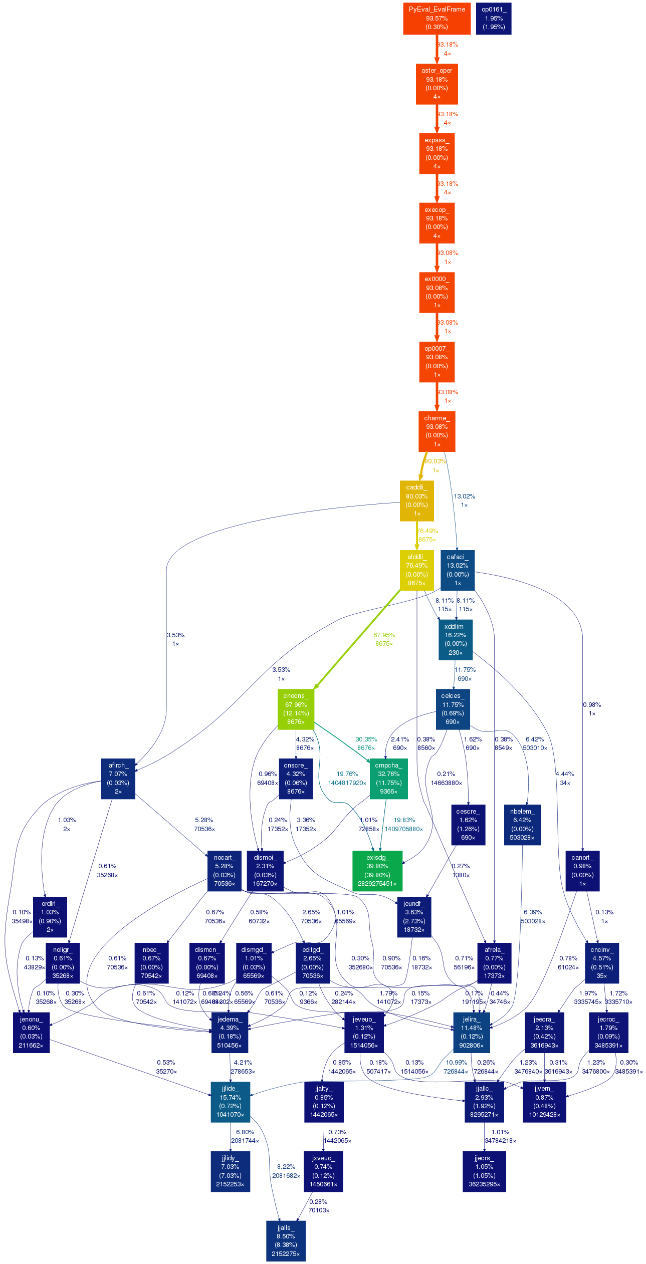
Figure 1: call graph generated with gprof2dot